
RESEARCH ARTICLE
A Methodology to Identify the Hinterland for Freight Ports by Transportation Cost Functions
Domenico Gattuso1, Gian Carla Cassone1, Domenica Savia Pellicanò1, *
Article Information

Identifiers and Pagination:
Year: 2023Volume: 17
E-location ID: e187444782212301
Publisher ID: e187444782212301
DOI: 10.2174/18744478-v17-e230109-2022-26
Article History:
Received Date: 13/7/2022Revision Received Date: 21/11/2022
Acceptance Date: 2/12/2022
Electronic publication date: 24/01/2023
Collection year: 2023

open-access license: This is an open access article distributed under the terms of the Creative Commons Attribution 4.0 International Public License (CC-BY 4.0), a copy of which is available at: https://creativecommons.org/licenses/by/4.0/legalcode. This license permits unrestricted use, distribution, and reproduction in any medium, provided the original author and source are credited.
Abstract
Introduction:
The competitiveness of a port depends on hinterland characteristics, among other factors. In particular, hinterland accessibility and efficient inland logistics are key factors in ensuring the speed of goods flows. The port systems have to be configured as an efficient and logistically effective interface between oceanic maritime trade and inland trade.
The paper has been elaborated starting from research carried out in the European ISTEN project (Integrated and Sustainable Transport in the Efficient Network), aiming to improve the intermodal connections among the ports of the Adriatic-Ionian area and the ports and their hinterlands.
Objective:
The objective of the work is to propose an original approach for identifying the port hinterland based on the evaluation of transport times and costs in the whole supply chain (from the origin in the foreland zone to a final destination in the hinterland).
Methods:
The analyses have been carried out by considering separately the transport time and monetary cost components and generalized transport cost. The methodology involves wide research of data and careful analysis of the port hinterland connectivity. An analytical application is proposed in order to identify and compare the potential hinterlands of two Italian ports, Gioia Tauro and Genoa.
Results:
The results of the proposed analyses show that the geographical distribution of the port hinterlands changes significantly in relation to the reference drivers in terms of monetary cost and time along the intermodal international paths; this has led to further analyses considering the transport generalized cost which has integrated into travel time and monetary cost.
Conclusion:
The aim of the proposed approach is to overcome the limits of the methodologies of the sector based on geographical characteristics that focus attention only on market aspects considering marginally the transport component. The methodology is transferable to other contexts and other types of freight interchange nodes by adapting the cost functions.
1. INTRODUCTION
The activity level of the ports is closely related to the dynamics of the hinterland, subject to continuous changes in terms of accessibility and logistics. The competitiveness of a port depends on several factors as the network transport supply to move freight towards the inland final destination [1]. According to some researchers, hinterland connectivity is the second most important factor driving the port competitiveness, after costs to cross the port [2, 3]. The ability to penetrate the hinterland is realized through efficient inland logistics and connections able to guarantee the speed of goods flows. Ports have to be configured as an efficient and logistically effective interface between oceanic maritime trade and inland trade which have different characteristics, dimensions and rhythms.
Some analyses emerging from the COREALIS research project [4] show the impact that a mega container ship (14,000 TEUs) can give on a port hinterland (Fig. 1). Assuming 8,000 TEUs are unloaded in port, of these 4,000 TEUs are destined to the hinterland (10% by rail and 90% by road), 11 trains and about 2,500 trucks would be needed, with a great impact on hinterland in terms of traffic and freight flows.
The concept of port hinterland has been treated within the European ISTEN project (Interreg Programme VB) by the authors and a specific bibliographic analysis proposed [5].
There are many definitions of ports hinterland. The first definition of the port hinterland was provided in 1938 by Sargent as “the area served by a port” [6]. According to some other authors, the hinterland is a land space on which a port sells its services and interacts with its customers or a market area; other researchers define the hinterland as the area in which a port has a monopolistic position, i.e. the inner region provided by a port [7-9].
The port hinterland is made up of two parts (Fig. 2): the main hinterland and the competitive margin hinterland [10]. The main hinterland is the market area surrounding the port; it is a terrestrial space on which a port sells its services and interacts with its users. It represents the regional market share that the terminal owns, compared to other terminals that serve the same region. It brings together all the customers directly connected to the terminal and the land areas from which it draws and to which it distributes traffic. The competitive hinterland is the market area in which the port must compete more closely with the others for the companies.
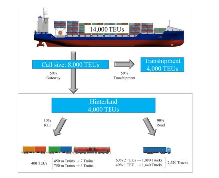 |
Fig. (1). Impact on hinterland generated by a mega containership port call [4]. |
 |
Fig. (2). Port hinterland types [10]. |
The main hinterland of a port is generally continuous. The density of hinterland origins or destination of a port decreases with distance. Hinterland “islands” can exist far from the port through the use of intermodal connections that allow the port to reach a competitive advantage in terms of costs and services compared to rival ports.
The hinterland can be further classified in relation to the kind of managed freights; in fact, each type of freight originates from a particular supply chain with specific spatial relationships.
A hinterland can have three basic sub-components: macro-economic, physical and logistical. The macro-economic hinterland tries to identify which factors are shaping transport demand, particularly in a global setting. The physical hinterland considers the nature and extension of the transport supply, both from a modal and intermodal perspective. Finally, the logistical hinterland is related to the organization of the flows [11].
Table 1 summarizes the main characteristics of the hinterland sub-components with particular reference to the transport supply sub-component. Transportation costs have been added as attributes time and cost reduction has been considered as a challenge.
| - | Hinterland | ||
|---|---|---|---|
| Macro-economic | Physical | Logistical | |
| Concept | Transport Demand | Transport Supply | Flows |
| Elements | Logistical sites as part of Global Commodity Chains | • Transport links • Terminals |
• Modes • Timing • Punctuality • Frequency |
| Attributes | • Interest rates • Exchange rates • Prices • Savings • Production • Debt |
• Capacity • Corridors • Terminals • Physical assets |
• Added value • Tons km • TEUs • Added value • ICT |
| Challenge | International division of production and consumption | Additional capacity (modal and intermodal) |
Supply chain Management |
The characteristics and dimensions of the port hinterland depend on many factors as:
- The type of moved freight, for example, for perishable goods, the time has great importance and the port hinterland is made up of the areas that can be reached in a time window compatible with their conservation [12];
- The degree of land connectivity, linked to intermodal transport services capable to guarantee the goods distribution in an efficient, reliable, rapid and economical way;
- The maritime connectivity which affects transport costs on the foreland side and consequently on the hinterland size; in fact, if the cost to reach a port is low, the number of shipping companies increases and the extension of the port hinterland increases too;
- The institutional and bureaucratic aspects as well as the presence of Special Economic Zones.
Many of these factors are not stable over time but may undergo intra-periodic (within the same period) and inter-periodic (among different periods) variations caused by changing local and global commercial, economic and geopolitical conditions.
It is important to study and analyse the port hinterland relationship in order to improve market access through the development of trade corridors, the fluidity of trade and integration into a wider logistics network.
One aspect of the analysis concerns the identification of the port's hinterlands and the definition of their dimensions; it is a theoretically complex issue due to factors such as:
- The hinterland can only be evaluated in relation to other ports as it is made up of all the areas where a port has generalized transport costs that are competitive with respect to other ports;
- The hinterland differs by type of cargo, type of stakeholder and destination abroad;
- The hinterland is not stable over time.
The paper is divided into three parts beyond the introduction and conclusions. In the first one, a state of the art model useful for the identification of the port hinterland is presented; in the second part, the proposed approach of the research and the methodology are described; the attention is focused on the cost functions useful for determining the generalized transport costs. Finally, an analytical application is proposed in order to identify and compare the potential hinterlands of two Italian container ports, Gioia Tauro and Genoa.
2. MATERIALS AND METHODS
2.1. Literature Review
Some overview of approaches for defining and analysing port hinterlands are in the literature of the sector [13]. From the first definition of port hinterland in 1938 [6] to the introduction of container transport, where researchers deepened the relationship between foreland and hinterland of ports, highlighting the need to introduce new approaches [14, 15]; until recent years, where port regionalization and contemporary port hinterland relations have suggested advanced methods including additional parameters for the analysis of the complex spatial structure of the contemporary port hinterland [16].
Some authors [17-20] have proposed quantitative models for defining the hinterland of a port.
Meng et al. [17] have developed a discreet choice theory-based approach to estimating boundaries of the probabilistic hinterland of a port for intermodal freight transport operations. The authors have defined the probabilistic hinterland of a port and derived its mathematical formulation by assuming that transportation costs or times of all available intermodal routes from an origin to a destination are multivariate and normally distributed. A Monte Carlo simulation-based algorithm has been developed in the research in order to graphically depict the port hinterland boundary with respect to a given probability value.
Hintjens [18, 19] has defined the attractiveness of a port A (PA) from hinterland connectivity as follows:
 |
(1) |
where HCA represents the connection cost to the hinterland, OCA is the cost of foreland connection including the cost of port operations, HCi and OCi are the corresponding costs related to port i in competition with port A, α is a parameter of the model. To carry out the shipment, it is possible to use a single-mode or multimodal transport; in the second case, it is necessary to consider the costs of loading unit transhipment. HCi is the sum of the costs of all used hinterland transport modes ck and the transhipment costs ctk-1 from each mode k:
 |
(2) |
The model proposed by Arvis et al. [20] has provided a first indication of the port hinterland based on three variables: the road distance, the sea distance and the maritime connectivity with the reference region. These variables have been evaluated in relation to the same distances for competing ports. The model has proposed the evaluation of a utility (Up,os,h) connected to the use of a port p for goods that must be transferred from region os (overseas region) to region h (hinterland region):
 |
(3) |
where RDp,h is the road distance between port p and hinterland region h; MDp,os is the maritime distance between port p and a certain world region; MCp is the maritime connectivity of the port p; α1, α2 and α3 are models’ parameters; αp,h0 is an error term.
It is possible to identify the port hinterland with reference to a specific transportation mode, for example using the theory of influence areas that allow to compare road transport with intermodal transport and to evaluate the influence area of intermodal transport and so the potential distant hinterland generated by the activation of an intermodal corridor.
This theory is an approach for choosing the location of a terminal and involves the analysis of the considered area to identify specific zones of influence within which it is convenient, in terms of lower overall transport cost, to use that particular terminal instead another.
In general, the procedure to identify the zone of influence can be divided into three phases:
- Development of decision-making processes that lead freight transport operators to choose combined transport;
- Identification of the savings obtainable from the choice of combined transport;
- Comparison of the different alternatives through the use of multi-objective procedures.
The larger the zone of influence, the greater the number of users potentially attracted by the node, in this case, the port, through the use of given modes of transport.
The sector literature models are essentially based on economic considerations that aim to identify potential markets in the hinterland for commercial ports. In some cases, the whole transport chain is not considered and the time and cost of transport variables are considered only marginally. The proposed methodological approach tries to overcome these limits; in particular, for the definition of the hinterland extension of a port, the generalized cost of transport with reference to the whole supply chain (foreland-hinterland) is considered. The developed methodological approach is described in detail in the following paragraph.
2.2. Port hinterland identification: methodological approach
The proposed methodological approach for identifying the port's hinterland is based on considerations relating to freight transport costs and refers to the whole supply chain from the origin (foreland - F) to destination (hinterland - H) in order to identify the potential hinterland in relation to a specific foreland geographical area.
In fact, port connectivity has three interdependent dimensions: maritime connectivity (also referred to as shipping networks) from the foreland origin port; port efficiency, which refers to the performance of the destination; and hinterland connectivity, which involves multiple players and institutions contributing to economic development and exploiting maritime supply chains (Fig. 3).
Costs evaluation can be made by considering the time and monetary cost of transport or referring to generalized transport cost. In the first case, it is possible to evaluate the incidence of the single factor simplifying the phenomena interpretation by the operators; in the second case, a synthetic indicator can be obtained, useful for simulation and planning studies.
The analysis based on generalized transport cost has been found to be more significant and thus it is proposed. The steps for identifying the ports hinterland can be the following (Fig. 4).
 |
Fig. (3). Dimensions of trade connectivity. |
 |
Fig. (4). Methodological approach for hinterland identification. |
- Zoning of foreland (F) and potential hinterland (H);
- Evaluation of transport times and costs for each F-H pair considering the crossing of the port P;
- Evaluation of the generalized transport cost, given the freight type and the relative Value of Time (VoT);
- Identification of the hinterland or the region for which, in relation to the considered Foreland area, there is a generalized cost of transport belonging to a specific threshold value.
The transport generalised cost can be evaluated starting from travel time and monetary cost. The door-to-door time and cost can be calculated, considering the three main phases of the freight path, by the following expressions:
 |
(4) |
where tM and CM are time and cost of maritime transport; tP and CP are respectively time and cost in a port node; tH and CH are the time and cost of hinterland transport by rail.
The proposed analysis refers to the supply chain of non-perishable goods; the perishable goods have heavy transport constraints linked to the cold chain which have been neglected in this phase of the study.
The costs (time and money) associated with maritime transport depend on many factors. The maritime travel time (tM) depends on the type of route (R), ship (S), intermediate stops (NP), travelled distance (L), and cruising speed during navigation in the sea (vc):
 |
(5) |
This component can be extracted from the services supply of maritime companies or estimated in relation to maritime distance, average navigation speed, and followed the path.
The cost of transport by sea (CM) is a function of variables such as distance (L), used container type (Tc), transport type (Tt), the value of the goods (Vg), and goods kind (Tg):
 |
(6) |
This component can be extracted from the service supply of the maritime companies.
For railway transport in the hinterland, the time (tH) and monetary cost (CH) can be estimated using the following aggregate models:
 |
(7) |
 |
(8) |
where L is the distance (km); vr is the commercial speed for freight trains (km/h); β is a unit cost parameter (€/t·km); Q is the quantity of moved freight (t). The commercial speed (vr) and the β parameter vary according to the geographical area of reference.
The evaluation of the temporal and monetary costs at interchange nodes, and in particular at the ports, is not easy; costs and times depend on a large set of different factors. It is useful to take into account the operations of the equipment to serve the ships and move containers, and to consider the loyalty relationships among operators and terminals.
In general, the costs to cross the port node (CP) consist of the Terminal Handling Charges (CTHC), the Storage Charges (CSC) and the Container Handling Rates (CCHR):
 |
(9) |
The CTHC represents the cost related to the loading/unloading of the container on/from the ship and it is charged to the shipping company by the terminal operator. THC is not considered a surcharge, but an ancillary charge, similar to documentation fees. Generally, it varies according to the reference trade route.
The CSC represents the storage cost for port usage or terminal depot or inland container yard facilities. This charge is levied by the port or the terminal to the shipping line. It depends on the direction of the commercial flow (import/export), the type of contract between the company and the terminal operator, and the kind of container stored (20’, 40’, dry, reefer, etc.) and it is proportional to the holding time of the container at the node. Generally, for the first week, it is zero and increases after, week by week.
Finally, the CCHR is the cost to move the container between the different areas of the terminal towards road/railway and vice versa. This cost depends on the number of movements and the kind of handling vehicle. The values assumed for the CCHR are 40 and 24 €/move, for sea-railway and sea-road interchange (our survey for port terminal operators), respectively.
Ultimately, the generalized transport cost (Cg) can be evaluated by using the following expression:
 |
(10) |
where CF-H is the monetary cost [€], VoT is the value of time [€/h], and tF-H is the time [h]. A high variability in VoT has been observed among studies in literature; it is assumed to be equal to 1.43 €/(t h) for non-perishable goods, according to FDOT [21].
The generalized transport cost has to be related to threshold values (upper bounds) in order to identify the hinterland for each port from different forelands. The upper bound can be calculated starting from the average generalized transport cost from each foreland to each destination port. Comparing the value obtained for Gioia Tauro and Genoa ports, the upper bound is assumed as the maximum average value; the potential hinterland is defined as a set of inland regions for which the value of generalized transport cost does not exceed the threshold.
2.3. Database for Application
The materials used for the research consist of a database structured starting from data provided by the companies and literature studies. The database refers, in particular, to two European ports, Gioia Tauro and Genoa, in Italy. As a foreland origin, the Chinese port of Shanghai has been adopted.
The evaluation of travel times along the routes is made by taking reference to the navigation times of some of the major shipping companies (Table 2) or assuming the distances without intermediate stops and an average speed vs of a container ship (Table 3).
The monetary costs of transport by sea (CM) have been hired with reference to the data of the shipping companies (Table 4).
| Shipping Company | O-D | Distance (km) | NP* | Time (Days) |
|---|---|---|---|---|
| MSC | Shanghai – Gioia Tauro | 15,148 | 0 | 26 |
| Shanghai – Genoa | 16,057 | 1 | 31 | |
| MAERSK | Shanghai – Gioia Tauro | 15,148 | 0 | 25 |
| Shanghai – Genoa | 16,057 | 1 | 37 |
| O-D | Distance (km) |
vs (km/h) |
Travel Time (days) |
|---|---|---|---|
| Shanghai – Gioia Tauro | 15,148 | 24 | 26 |
| Shanghai – Genoa | 16,057 | 24 | 28 |
| Good Type | Container Type | Transport Type |
Cost (€/TEU) |
|||
|---|---|---|---|---|---|---|
| P | No P | 20’ | 40’ | FCL | LCL | |

|
- |
|
- |
|
- | 1,087 |
|
|
- |
|
- | - |
|
1,400 |
|
|
- | - |
|
|
- | 1,278 |
|
|
- | - |
|
- |
|
1,646 |
|
|
|
- |
|
- | 963 | |
|
|
|
- | - |
|
1,239 | |
|
|
- |
|
|
- | 1,131 | |
|
|
- |
|
- |
|
1,456 | |
For railway transport in the hinterland, the commercial speed (vr) has been assumed starting from the data of the main railway companies; β has been defined on the basis of some literature works (table 5 and 6).
| Geographic Area | vr (km/h) |
|---|---|
| Italy | 50 |
| Central/Northern Europe | 60 |
| Eastern Europe | 15 |
| Geographic Area | β (€/t·km) |
|---|---|
| Italy to Germany (our processing on [23]) | 0.05 |
| Into Germany [24] | 0.06 |
| Eastern Europe (our processing on [21]) | 0.04 |
About the evaluation of the times and monetary costs at interchange nodes, the values of dwell times (tP) through some ports for interchange sea-rail are given in Table 7. These values have been estimated starting from a survey realized among shippers.
| Port | Time (Days) |
|---|---|
| Gioia Tauro | 2 - 5 |
| Genoa | 2 - 4 |
| Rotterdam | 1 – 2 |
| Piraeus | 4 – 7 |
| Shanghai | 2 – 3 |
According to the data published by the Italy Bank, Table 8 shows the unitary values assumed for the CTHC (cost for 1 TEU).
|
Geographic Area (Import/Export) |
Italian/European Ports | Foreign Ports |
|---|---|---|
| Mediterranean | 181 | 180 |
| Middle East | 160 | 180 |
| Africa | 158 | 145 |
| USA and Canada | 170 | 433 |
| Central/South America (Pacific) | 190 | 116 |
| South America (Atlantic) | 189 | 116 |
| India | 158 | 41 |
| China and South East Asia | 160 | 150 |
| Japan and Far East | 160 | 187 |
| Oceania | 165 | 187 |
| Average | 169.1 | 173.5 |
The proposed approach is conditioned by the difficulty of finding and updating the numerous parameters involved, often depending on the spatial-temporal contexts and the structure of markets and logistic chains.
3. RESULTS
The proposed methodology has been applied to the two biggest Italian ports in container traffic, Gioia Tauro and Genoa, in order to identify their potential hinterland and to compare them. These two ports have different characteristics; in particular, whereas transshipment in the port of Genoa represents around 12% of total activities, the port of Gioia Tauro is dedicated exclusively to transshipment operations.
The Genoa port is one of the main ports in the Mediterranean basin and a fundamental element for the industrial activities in Northern Italy. It is configured as a multi-function port, with many terminals equipped to accommodate all types of traffic: containers, general cargo, perishable products, metals, forestry, solid and liquid bulk, petroleum products, and passengers. A part of the port offers highly specialized complementary services as shipbuilding and repairs, technology and information technology.
Gioia Tauro port is an Italian transshipment hub, it has a central location in the trades among Asia, the Mediterranean Sea and the East Coast of the United States. For this reason, the port has a relevant role in intercontinental maritime traffic. Its location represents a meeting point between the East-West Sea lines and Europe. In relation to international trade fostering the route of the Suez Canal, the port has potential in relation to large communication plans and business development. The traffic affecting the port of Gioia Tauro mainly concerns the transshipment of containers and vehicles. A railway gateway has recently been built near the port; it is today operational and regular connections are guaranteed through the Thyrrenian railway to different Italian regions.
In order to carry out the analyses, foreland has been divided into 8 large zones (Middle East; India, South East Asia; China and Japan; Southern Africa; South America and West Africa; USA/Canada and Central America; Oceania) represented through a representative container port in a barycentric position. Italy has been considered a potential hinterland and it has been divided into 18 zones corresponding to the Italian regions (excluding the islands), represented through sites corresponding to regional railway freight stations.
The evaluations have been made taking into consideration a 20’ container loaded with non-perishable goods worth € 2,000, for a total mass of 25 tons.
Table 9 shows the distances by sea between the foreland areas and the ports of Gioia Tauro and Genoa; Table 10 shows the distances by rail between the ports of Gioia Tauro and Genoa and the hinterland zones. table 11-16 show the matrixes of times, monetary costs and generalized transport costs for F-H pairs through the Gioia Tauro and Genoa container ports.
|
Distance from Gioia Tauro |
Distance from Genoa | |||
|---|---|---|---|---|
| Foreland Zone | Nautical Miles | Km | Nautical Miles | Km |
| 1. Middle East | 3,984 | 7,378 | 4,475 | 8,288 |
| 2. Southern Africa | 6,118 | 11,331 | 5,937 | 10,995 |
| 3. India | 4,965 | 9,195 | 5,456 | 10,105 |
| 4. South East Asia | 5,942 | 11,005 | 6,433 | 11,914 |
| 5. China and Japan | 8,179 | 15,148 | 8,670 | 16,057 |
| 6. Oceania | 8,427 | 15,607 | 8,918 | 16,516 |
| 7. USA, Canada and Central America | 4,513 | 8,358 | 4,332 | 8,023 |
| 8. South America and West Africa | 5,527 | 10,236 | 5,346 | 9,901 |
| Hinterland Zone |
Distance from Gioia Tauro (km) |
Distance from Genoa (km) |
|---|---|---|
| Abruzzo | 471 | 478 |
| Basilicata | 246 | 721 |
| Calabria | 71 | 861 |
| Campania | 302 | 599 |
| Emilia Romagna | 847 | 120 |
| Friuli Venezia Giulia | 854 | 392 |
| Lazio | 538 | 353 |
| Liguria | 905 | 33 |
| Lombardy | 957 | 155 |
| Marche | 641 | 359 |
| Molise | 364 | 564 |
| Piedmont | 1,489 | 60 |
| Puglia | 312 | 743 |
| Toscany | 738 | 146 |
| Trentino Alto Adige | 936 | 252 |
| Umbria | 536 | 363 |
| Valle d'Aosta | 1,077 | 195 |
| Veneto | 860 | 292 |
| Hinterland Zone | ||||||||||||||||||
|---|---|---|---|---|---|---|---|---|---|---|---|---|---|---|---|---|---|---|
| Foreland Zone | Abruzzo | Basilicata | Calabria | Campania | Emilia R. | Friuli V.G. | Lazio | Liguria | Lombardy | Marche | Molise | Piedmont | Puglia | Tuscany | Trentino A.G. | Umbria | Valle d'Aosta | Veneto |
| 1 | 19.2 | 19.0 | 18.9 | 19.1 | 19.4 | 19.4 | 19.2 | 19.5 | 19.5 | 19.3 | 19.1 | 19.9 | 19.1 | 19.4 | 19.5 | 19.2 | 19.6 | 19.4 |
| 2 | 26.7 | 26.5 | 26.4 | 26.6 | 27.0 | 27.0 | 26.8 | 27.1 | 27.1 | 26.9 | 26.6 | 27.6 | 26.6 | 26.9 | 27.1 | 26.8 | 27.2 | 27.1 |
| 3 | 29.7 | 29.5 | 29.4 | 29.6 | 30.0 | 30.0 | 29.8 | 30.1 | 30.1 | 29.9 | 29.6 | 30.6 | 29.6 | 29.9 | 30.1 | 29.8 | 30.2 | 30.1 |
| 4 | 17.7 | 17.5 | 17.4 | 17.6 | 18.0 | 18.0 | 17.8 | 18.1 | 18.1 | 17.9 | 17.6 | 18.6 | 17.6 | 17.9 | 18.1 | 17.8 | 18.2 | 18.1 |
| 5 | 28.2 | 28.0 | 27.9 | 28.1 | 28.4 | 28.4 | 28.2 | 28.5 | 28.5 | 28.3 | 28.1 | 28.9 | 28.1 | 28.4 | 28.5 | 28.2 | 28.6 | 28.4 |
| 6 | 31.7 | 31.5 | 31.4 | 31.6 | 32.0 | 32.0 | 31.8 | 32.1 | 32.1 | 31.9 | 31.6 | 32.6 | 31.6 | 31.9 | 32.1 | 31.8 | 32.2 | 32.1 |
| 7 | 23.7 | 23.5 | 23.4 | 23.6 | 24.0 | 24.0 | 23.8 | 24.1 | 24.1 | 23.9 | 23.6 | 24.6 | 23.6 | 23.9 | 24.1 | 23.8 | 24.2 | 24.1 |
| 8 | 35.7 | 35.5 | 35.4 | 35.6 | 36.0 | 36.0 | 35.8 | 36.1 | 36.1 | 35.9 | 35.6 | 36.6 | 35.6 | 35.9 | 36.1 | 35.8 | 36.2 | 36.1 |
| Hinterland Zone | ||||||||||||||||||
|---|---|---|---|---|---|---|---|---|---|---|---|---|---|---|---|---|---|---|
| Foreland Zone | Abruzzo | Basilicata | Calabria | Campania | Emilia R. | Friuli V.G. | Lazio | Liguria | Lombardy | Marche | Molise | Piedmont | Puglia | Tuscany | Trentino A.G. | Umbria | Valle d'Aosta | Veneto |
| 1 | 21.8 | 22.0 | 22.1 | 21.9 | 21.5 | 21.8 | 21.7 | 21.5 | 21.6 | 21.7 | 21.9 | 21.5 | 22.0 | 21.6 | 21.6 | 21.7 | 21.6 | 21.7 |
| 2 | 26.0 | 26.2 | 26.3 | 26.1 | 25.7 | 25.9 | 25.9 | 25.7 | 25.8 | 25.9 | 26.1 | 25.7 | 26.2 | 25.7 | 25.8 | 25.9 | 25.8 | 25.9 |
| 3 | 32.4 | 32.6 | 32.7 | 32.5 | 32.1 | 32.3 | 32.3 | 32.0 | 32.1 | 32.3 | 32.5 | 32.1 | 32.6 | 32.1 | 32.2 | 32.3 | 32.2 | 32.2 |
| 4 | 19.0 | 19.2 | 19.3 | 19.1 | 18.7 | 18.9 | 18.9 | 18.6 | 18.7 | 18.9 | 19.0 | 18.6 | 19.2 | 18.7 | 18.8 | 18.9 | 18.7 | 18.8 |
| 5 | 30.3 | 30.5 | 30.6 | 30.4 | 30.0 | 30.2 | 30.2 | 29.9 | 30.0 | 30.2 | 30.4 | 29.9 | 30.5 | 30.0 | 30.1 | 30.2 | 30.1 | 30.1 |
| 6 | 33.4 | 33.6 | 33.7 | 33.5 | 33.1 | 33.3 | 33.3 | 33.1 | 33.2 | 33.3 | 33.5 | 33.1 | 33.6 | 33.1 | 33.2 | 33.3 | 33.2 | 33.3 |
| 7 | 22.9 | 23.1 | 23.2 | 23.0 | 22.6 | 22.8 | 22.8 | 22.5 | 22.6 | 22.8 | 23.0 | 22.5 | 23.1 | 22.6 | 22.7 | 22.8 | 22.7 | 22.7 |
| 8 | 34.7 | 34.9 | 35.0 | 34.8 | 34.4 | 34.6 | 34.5 | 34.3 | 34.4 | 34.6 | 34.7 | 34.3 | 34.9 | 34.4 | 34.5 | 34.6 | 34.4 | 34.5 |
| Hinterland Zone | ||||||||||||||||||
|---|---|---|---|---|---|---|---|---|---|---|---|---|---|---|---|---|---|---|
| Foreland Zone | Abruzzo | Basilicata | Calabria | Campania | Emilia R. | Friuli V.G. | Lazio | Liguria | Lombardy | Marche | Molise | Piedmont | Puglia | Tuscany | Trentino A.G. | Umbria | Valle d'Aosta | Veneto |
| 1 | 1,811 | 1,506 | 1,269 | 1,582 | 2,321 | 2,330 | 1,902 | 2,399 | 2,470 | 2,041 | 1,666 | 3,191 | 1,595 | 2,173 | 2,441 | 1,899 | 2,632 | 2,338 |
| 2 | 2,479 | 2,174 | 1,937 | 2,250 | 2,989 | 2,998 | 2,570 | 3,068 | 3,138 | 2,710 | 2,334 | 3,859 | 2,264 | 2,841 | 3,110 | 2,567 | 3,301 | 3,007 |
| 3 | 1,534 | 1,229 | 992 | 1,305 | 2,043 | 2,053 | 1,625 | 2,122 | 2,192 | 1,764 | 1,389 | 2,913 | 1,318 | 1,896 | 2,164 | 1,622 | 2,355 | 2,061 |
| 4 | 1,522 | 1,217 | 980 | 1,293 | 2,032 | 2,041 | 1,613 | 2,110 | 2,181 | 1,752 | 1,377 | 2,902 | 1,306 | 1,884 | 2,152 | 1,610 | 2,343 | 2,049 |
| 5 | 1,822 | 1,517 | 1,279 | 1,592 | 2,331 | 2,341 | 1,912 | 2,410 | 2,480 | 2,052 | 1,676 | 3,201 | 1,606 | 2,183 | 2,452 | 1,910 | 2,643 | 2,349 |
| 6 | 2,059 | 1,754 | 1,517 | 1,830 | 2,568 | 2,578 | 2,150 | 2,647 | 2,718 | 2,289 | 1,914 | 3,439 | 1,843 | 2,421 | 2,689 | 2,147 | 2,880 | 2,586 |
| 7 | 1,727 | 1,422 | 1,185 | 1,498 | 2,237 | 2,246 | 1,818 | 2,315 | 2,386 | 1,958 | 1,582 | 3,107 | 1,512 | 2,089 | 2,357 | 1,815 | 2,548 | 2,254 |
| 8 | 1,753 | 1,448 | 1,211 | 1,524 | 2,262 | 2,272 | 1,843 | 2,341 | 2,411 | 1,983 | 1,608 | 3,132 | 1,537 | 2,114 | 2,383 | 1,841 | 2,574 | 2,280 |
| Hinterland | ||||||||||||||||||
|---|---|---|---|---|---|---|---|---|---|---|---|---|---|---|---|---|---|---|
| Foreland Zone | Abruzzo | Basilicata | Calabria | Campania | Emilia R. | Friuli V.G. | Lazio | Liguria | Lombardy | Marche | Molise | Piedmont | Puglia | Tuscany | Trentino A.G. | Umbria | Valle d'Aosta | Veneto |
| 1 | 1,830 | 2,159 | 2,349 | 1,994 | 1,345 | 1,713 | 1,661 | 1,227 | 1,392 | 1,669 | 1,946 | 1,263 | 2,189 | 1,380 | 1,524 | 1,674 | 1,446 | 1,578 |
| 2 | 2,505 | 2,834 | 3,024 | 2,669 | 2,019 | 2,388 | 2,335 | 1,901 | 2,067 | 2,343 | 2,621 | 1,938 | 2,864 | 2,055 | 2,198 | 2,349 | 2,121 | 2,252 |
| 3 | 1,550 | 1,880 | 2,069 | 1,714 | 1,065 | 1,434 | 1,381 | 947 | 1,112 | 1,389 | 1,667 | 984 | 1,909 | 1,100 | 1,244 | 1,394 | 1,167 | 1,298 |
| 4 | 1,538 | 1,868 | 2,057 | 1,702 | 1,053 | 1,422 | 1,369 | 935 | 1,100 | 1,377 | 1,655 | 972 | 1,897 | 1,088 | 1,232 | 1,382 | 1,155 | 1,286 |
| 5 | 1,841 | 2,170 | 2,360 | 2,005 | 1,355 | 1,724 | 1,671 | 1,237 | 1,403 | 1,679 | 1,957 | 1,274 | 2,200 | 1,391 | 1,534 | 1,685 | 1,457 | 1,588 |
| 6 | 2,080 | 2,409 | 2,599 | 2,244 | 1,595 | 1,964 | 1,911 | 1,477 | 1,642 | 1,919 | 2,197 | 1,514 | 2,439 | 1,630 | 1,774 | 1,924 | 1,697 | 1,828 |
| 7 | 1,745 | 2,075 | 2,264 | 1,909 | 1,260 | 1,629 | 1,576 | 1,142 | 1,308 | 1,584 | 1,862 | 1,179 | 2,104 | 1,295 | 1,439 | 1,589 | 1,362 | 1,493 |
| 8 | 1,771 | 2,100 | 2,290 | 1,935 | 1,286 | 1,654 | 1,602 | 1,168 | 1,333 | 1,610 | 1,888 | 1,205 | 2,130 | 1,321 | 1,465 | 1,615 | 1,387 | 1,519 |
| Hinterland | ||||||||||||||||||
|---|---|---|---|---|---|---|---|---|---|---|---|---|---|---|---|---|---|---|
| Foreland Zone | Abruzzo | Basilicata | Calabria | Campania | Emilia R. | Friuli V.G. | Lazio | Liguria | Lombardy | Marche | Molise | Piedmont | Puglia | Tuscany | Trentino A.G. | Umbria | Valle d'Aosta | Veneto |
| 1 | 18.3 | 17.8 | 17.5 | 17.9 | 19.0 | 19.0 | 18.4 | 19.1 | 19.2 | 18.6 | 18.1 | 20.2 | 18.0 | 18.8 | 19.2 | 18.4 | 19.4 | 19.0 |
| 2 | 25.4 | 24.9 | 24.6 | 25.1 | 26.2 | 26.2 | 25.5 | 26.3 | 26.4 | 25.8 | 25.2 | 27.5 | 25.1 | 26.0 | 26.4 | 25.5 | 26.7 | 26.2 |
| 3 | 27.0 | 26.6 | 26.2 | 26.7 | 27.8 | 27.8 | 27.2 | 27.9 | 28.0 | 27.4 | 26.8 | 29.1 | 26.7 | 27.6 | 28.0 | 27.2 | 29.1 | 27.8 |
| 4 | 16.7 | 16.3 | 15.9 | 16.4 | 17.5 | 17.5 | 16.9 | 17.6 | 17.7 | 17.1 | 16.5 | 18.8 | 16.4 | 17.3 | 17.7 | 16.9 | 18.0 | 17.5 |
| 5 | 26.0 | 25.6 | 25.2 | 25.7 | 26.7 | 26.7 | 26.1 | 26.8 | 26.9 | 26.3 | 25.8 | 28.0 | 25.7 | 26.5 | 26.9 | 26.1 | 27.6 | 26.8 |
| 6 | 29.3 | 28.8 | 28.5 | 28.9 | 30.1 | 30.1 | 29.4 | 30.2 | 30.3 | 29.6 | 29.1 | 31.4 | 29.0 | 29.8 | 30.2 | 29.4 | 30.6 | 30.1 |
| 7 | 22.1 | 21.6 | 21.3 | 21.7 | 22.9 | 22.9 | 22.2 | 23.0 | 23.1 | 22.4 | 21.9 | 24.2 | 21.8 | 22.6 | 23.0 | 22.2 | 23.3 | 22.9 |
| 8 | 32.4 | 31.9 | 31.6 | 32.1 | 33.2 | 33.2 | 32.5 | 33.3 | 33.4 | 32.8 | 32.2 | 34.5 | 32.1 | 33.0 | 33.4 | 32.5 | 33.7 | 33.2 |
| Hinterland | ||||||||||||||||||
|---|---|---|---|---|---|---|---|---|---|---|---|---|---|---|---|---|---|---|
| Foreland Zone | Abruzzo | Basilicata | Calabria | Campania | Emilia R. | Friuli V.G. | Lazio | Liguria | Lombardy | Marche | Molise | Piedmont | Puglia | Tuscany | Trentino A.G. | Umbria | Valle d'Aosta | Veneto |
| 1 | 20.6 | 21.1 | 21.4 | 20.8 | 19.8 | 20.4 | 20.3 | 19.6 | 19.9 | 20.3 | 20.7 | 19.7 | 21.1 | 19.9 | 20.1 | 20.3 | 20.0 | 20.2 |
| 2 | 24.8 | 25.3 | 25.6 | 25.1 | 24.1 | 24.7 | 24.6 | 23.9 | 24.2 | 24.6 | 25.0 | 24.0 | 25.4 | 24.1 | 24.4 | 24.6 | 24.2 | 24.4 |
| 3 | 29.4 | 29.9 | 30.1 | 29.6 | 28.6 | 29.2 | 29.1 | 28.4 | 28.7 | 29.1 | 29.5 | 28.5 | 29.9 | 28.7 | 28.9 | 29.1 | 28.8 | 29.0 |
| 4 | 17.8 | 18.3 | 18.6 | 18.1 | 17.1 | 17.6 | 17.6 | 16.9 | 17.1 | 17.6 | 18.0 | 17.0 | 18.4 | 17.1 | 17.3 | 17.6 | 17.2 | 17.4 |
| 5 | 27.8 | 28.3 | 28.6 | 28.1 | 27.1 | 27.7 | 27.6 | 26.9 | 27.2 | 27.6 | 28.0 | 27.0 | 28.4 | 27.1 | 27.4 | 27.6 | 27.2 | 27.4 |
| 6 | 30.8 | 31.3 | 31.5 | 31.0 | 30.0 | 30.6 | 30.5 | 29.8 | 30.1 | 30.5 | 30.9 | 29.9 | 31.3 | 30.1 | 30.3 | 30.5 | 30.2 | 30.4 |
| 7 | 21.4 | 21.9 | 22.2 | 21.6 | 20.6 | 21.2 | 21.1 | 20.5 | 20.7 | 21.1 | 21.6 | 20.5 | 21.9 | 20.7 | 20.9 | 21.1 | 20.8 | 21.0 |
| 8 | 31.5 | 32.0 | 32.3 | 31.8 | 30.8 | 31.3 | 31.2 | 30.6 | 30.8 | 31.3 | 31.7 | 30.6 | 32.1 | 30.8 | 31.0 | 31.3 | 30.9 | 31.1 |
| Foreland Zone | Upper bound (€) |
|---|---|
| 1. Middle East | 20,337 |
| 2. Southern Africa | 25,832 |
| 3. India | 29,130 |
| 4. South East Asia | 17,595 |
| 5. China and Japan | 27,611 |
| 6. Oceania | 30,535 |
| 7. USA, Canada and Central America | 22,506 |
| 8. South America and West Africa | 32,827 |
Not having indications about the availability to pay by the field operators for reaching the final destination, the hinterland dimension has been defined considering an upper bound in relation to the average generalized transport cost from each foreland to each destination port. Comparing the values obtained for Gioia Tauro and Genoa ports, the upper bound has been assumed as the higher average value (Table 17); the potential hinterland is defined as the set of the region for which the generalized transport cost does not exceed this threshold.
An analysis of the results (Fig. 5) shows that the hinterland for the Gioia Tauro port is represented by the whole Italian Country for goods from the Middle East; whereas some regions of Northern Italy are excluded if the forelands are India (Piedmont, Val d’Aosta), China, Japan and Oceania (Piedmont, Val d’Aosta, Friuli Venezia Giulia), South East Asia (Piedmont, Val d’Aosta, Liguria, Lombardy, Trentino Alto Adige).
 |
Fig. (5). Potential Hinterland for Gioia Tauro and Genoa ports with reference generalized cost. |
The freight coming from South Africa, USA/Canada and Central America, South America and West Africa, landed in Gioia Tauro, will have Central and Southern Italy as a potential hinterland.
Concerning the hinterland of Genoa port, it consists of all the Italian regions if the goods come from South Africa, USA/Canada, Central America, South America and West Africa.
The forelands Oceania and China and Japan have a Genoa hinterland represented by Central-Northern Italy. The same situation occurs in the Middle East, India and South East Asia with the exception of the Italian region of Friuli Venezia Giulia.
4. DISCUSSION
Comparative analyzes are not easy in relation to the heterogeneity of sources and the variability over time of the transport supply, particularly in shipping.
From the analytical results obtained, it emerges that the hinterland dimension of each port is also linked to the accesses of ships to the Mediterranean basin, Suez (East), or Gibraltar (West).
In fact, it emerges that for goods crossing the Strait of Gibraltar (South Africa, USA/Canada and Central America, South America and West Africa) the port of Genoa is more attractive.
For the goods crossing the Suez Canal to reach their destination (from Middle East, India South East Asia, China and Japan, and Oceania), the Gioia Tauro port is more convenient, in fact, its hinterland is more extensive.
Gioia Tauro records a growing trend of transshipment traffic (since 2,4 million TEUs, in 2017, to about 3,1 million in 2021 and a forecast of 3,5 TEUs at the ned of 2022) and in the last years, a part of the traffic has been shifting to continental rail transport (2,5% expected for 2022). This trend could be greatly strengthened following the ongoing upgrading of the Adriatic-Ionian railway corridor, as highlighted in the ISTEN research, as the transit time towards Central Europe could become competitive with respect to that relating to maritime transport from Suez which today reaches ports of the European Northern range through the Strait of Gibraltar, the Atlantic Ocean and the English Channel.
Gioia Tauro and Genoa ports are configured as direct competitors; really Genoa port is currently more attractive as the Gioia Tauro port is affected by the bottlenecks related to railway intermodality and the Ionian-Adriatic railway corridor.
Further analysis has been made to evaluate the extension of the hinterland of the Rotterdam port. The hinterland of Rotterdam reaches Northern Italy in relation to the road and railway transport costs (time, cost or generalized cost), thanks to the high performance of the port (on average, the goods stop for 1 day at the port before being loaded on the wagons). The improvement in the performance of the Gioia Tauro port and the enhancement of the Adriatic-Ionian railway in progress would push probably its hinterland up to Central Europe.
CONCLUSION
The paper has proposed a methodology for identifying the hinterland of a port based on considerations relating to transport costs and times. The methodology has involved a careful analysis of port-hinterland connectivity. The port-hinterland corridors can develop differently depending on the regional economic conditions and their intensity on the territory, on the importance of ports at the regional level and the characteristics of the freight transport corridors on a local, regional, or national/transnational scale. The paper has proposed furthermore an application for the identification of the Gioia Tauro port hinterland in relation to the Genoa port.
The port of Gioia Tauro could be configured as a direct competitor of the Genoa port when its inland connections will be fully operational in the next future.
The results of the proposed analyses have shown that the geographical distribution of the port hinterlands changes significantly in relation to the values of the generalized transport cost which integrates into a single indicator the travel time and information relating to the monetary cost.
A proposed methodology is an original approach that allows overcoming the limits of the geographical approach that focuses attention only on market aspects and leaves aside the transport component. The methodology is transferable to other contexts and other types of freight interchange sites by adapting the cost functions appropriately.
The research is part of the activities carried out in the ISTEN project (Integrated and Sustainable Transport in the Efficient Network), financed by the ADRION Community Program, in the context of the Interreg EU Program, aiming to improve the intermodal connections among the maritime ports of the Adriatic-Ionian area and among the ports and their hinterlands. In evaluating the potential hinterland for the Gioia Tauro port, the use of railway Ionian-Adriatic corridor could have a positive impact and could increase its international role.
In recent years, there is a strong growth of the Gioia Tauro port in terms of rail connections with Central and Northern Italy. Also, in relation to the constant growth of containerized flows (since 2,4 million TEUs, in 2017, to about 3,1 million TEUs in 2021) and furthermore, to the continuous strengthening of transport infrastructures, in particular along the ADRION corridor (Adriatic-Ionian), growth is expected in the role of the Calabrian port in relations with Central Europe. This could lead to a greater competitiveness of this port and therefore to a greater extension of its hinterland on the European continent.
CONSENT FOR PUBLICATION
Not applicable.
AVAILABILITY OF DATA AND MATERIALS
Not applicable.
FUNDING
The research is part of the activities carried out in the ISTEN project (Integrated and Sustainable Transport in the Efficient Network), financed by the ADRION Community Program, in the context of the Interreg EU Program.
CONFLICT OF INTEREST
The authors declare that the paper has been elaborated after the end of Research in the Interreg ADRION Programme, a European Research Project (ISTEN - Integrated and Sustainable Transport in Efficient Network). Moreover, it represents an upgrade of a component of activity managed by the authors. Some parts of ISTEN's final publication are cited as a reference, but the authors declare there is no conflict of interest.
Dr. Domenico Gattuso is the Editorial Advisory Board Member for The Open Transportation Journal.
ACKNOWLEDGEMENTS
Declared none.
REFERENCES
| [1] | M. Acciaro, and A. Mckinnon, "Efficient hinterland transport infrastructure and services for large container ports", Working Paper: Port Investment and Container Shipping Markets, OECD, 2015p. 75. Available from: http://hdl.handle.net/10419/97076 |
| [2] | F. Parola, M. Risitano, M. Ferretti, and E. Panetti, "The drivers of port competitiveness: a critical review", Transp. Rev., vol. 37, no. 1, pp. 116-138, 2017. |
| [3] | R. Aronietis, E. Van de Voorde, and T. Vanelslander, "Port competitiveness determinants of selected European ports in the containerized cargo market", Paper presented at the European Transport Conference 2010, Glasgow. Scotland, United Kingdom., 2010. |
| [4] | C. Pérez, J. Freixanet, M. Giannini, and K. Hajredini, D.2.1: State of the Art of Port-Hinterland Connections, Working Paper: COREALIS Project. Horizon2020 Framework Programme, Available from: https://www.corealis.eu/wp-content/uploads/2020/02/D.2.1-State-of-the-Art-of-Port-Hinterland-Connections.pdf |
| [5] | D. Gattuso, and G.C. Cassone, "DT1.3.6 – ISTEN Toolbox, Working Paper: Integrated and Sustainable Transport in Efficient Network – ISTEN ", Available from: https://isten.adrioninterreg.eu/wp-content/uploads/2020/04/DT1.3.6_Final.pdf |
| [6] | A.J. Sargent, Seaports and Hinterlands.. Adam and Charles Black: London, 1938. |
| [7] | B. Slack, "Pawns in the game: ports in global transportation systems", Growth Change, vol. 24, no. 4, pp. 579-588, 1993. |
| [8] | H.A. van Klink, and G.C. van den Berg, "Gateways and intermodalism", J. Transp. Geogr., vol. 6, no. 1, pp. 1-9, 1998. |
| [9] | X. Fageda, "Load centres in the Mediterranean port range. Ports hub and ports gateway, Madrid,", Load centres in the Mediterranean port range., 2004. Available from: http://hdl.handle.net/10419/114874 |
| [10] | J.P. Rodrigue, The Geography of Transport Systems., 5th ed Routledge: London, 2020. |
| [11] | T. Notteboom, and J.P. Rodrigue, "Re-assessing port-hinterland relationships in the context of global supply chains", In: J. Wang, T. Notteboom, D. Olivier, and B. Slack, Eds., Ports, Cities, and Global Supply Chains.. Ashgate: Aldershot, 2017, pp. 51-68. |
| [12] | J. Hintjens, Cooperation between seaports concerning hinterland transport., Thesis for: Doctor in Applied Economics, Faculty of Business and Economics, Department of Transport and Regional Economics Antwerp, 2019. |
| [13] | E. Sdoukopoulos, and M. Boile, "Port-hinterland concept evolution: A critical review", J. Transp. Geogr., vol. 86, p. 102775, 2020. |
| [14] | N.R. Elliott, "Hinterland and foreland as illustrated by the Port of Tyne", Trans. Inst. Br. Geogr., vol. 47, no. 47, pp. 153-170, 1969. |
| [15] | R. Robinson, "The hinterland-foreland continuum: concept and methodology", Prof. Geogr., vol. 22, no. 6, pp. 307-310, 1970. |
| [16] | T. Notteboom, and J-P. Rodrigue, "Re-assessing port-hinterland relationships in the context of global commodity chains", In: J. Wang, T. Notteboom, D. Olivier, and B. Slack, Eds., Ports, Cities and Global Supply Chains.. Ashgate: Aldershot, 2007. |
| [17] | Q. Meng, X. Wang, and L. Miao, "Boundary estimation of probabilistic port hinterland for intermodal freight transportation operations", Proceedings of the 13th World Conference on Transport Research, 2013 Rio de Janeiro, Brazil |
| [18] | J. Hintjens, "A conceptual framework for cooperation in hinterland development between neighbouring seaport authorities", Marit. Policy Manage., vol. 45, no. 6, pp. 819-836, 2018. |
| [19] | J. Hintjens, E. van Hassel, T. Vanelslander, and E. Van de Voorde, "Port Cooperation and Bundling: A Way to Reduce the External Costs of Hinterland Transport", Sustainability (Basel), vol. 12, no. 23, p. 9983, 2020. |
| [20] | J.F. Arvis, V. Vesin, R. Carruthers, C. Ducruet, and P. de Langen, "Maritime networks, port efficiency, and hinterland connectivity in the mediterranean, working paper", International Bank for Reconstruction and Development/The World Bank, 2018. |
| [21] | FDOT- Florida Department of Transportation, Available from: https://www.fdot.gov/statistics/default.shtm |
| [22] | World Freight Rates, Available from: https://www.worldfreightrates.com/ |
| [23] | B. d’Italia, Indagine campionaria sui trasporti internazionali dell’Italia. Benchmark 2011, Working Paper Available from: https://www.bancaditalia.it/statistiche/tematiche/rapporti-estero/trasporti-internazionali/sintesi-indagini/indagine-trasporti11.pdf |
| [24] | Bundesnetzagentur, "Market analysis railway, working paper", Available from: https://www.bundesnetzagentur.de/SharedDocs/Downloads/EN/Areas/Rail/Downloads/MarketAnalysisRailway2016.pdf?__blob=publicationFile&v=3 |