All published articles of this journal are available on ScienceDirect.
Modelling of Friction Coefficient for Shoes Type LL By Means of Polynomial Fitting
Abstract
Introduction:
The paper describes the automatic procedure, implemented in UIC software TrainDy, for the simulation of friction coefficient of new LL shoes, used to avoid noise from freight traffic.
Method:
This procedure uses certified experimental data obtained at dynamometer bench as input data and computes a series of polynomials laws that describe the evolution of friction coefficient with speed, for different values of normal force between brake blocks and wheel and for different initial braking speeds.
Result:
Numerical results are compared against two series of experimental slip tests, carried on Trenitalia freight wagons, in terms of both stopping distances (for different starting speeds and loading conditions) and pressure in brake cylinder, speed and acceleration. Errors in terms of stopping distance are always below 5% whereas errors in terms of maximum acceleration are up to 20%.
1. INTRODUCTION
In Europe (EU 27 and Switzerland), freight trains are mainly equipped with brake blocks whereas disc brakes equip only more recent freight wagons with high performance (roughly 5% of wagons). Friction material of brake blocks wagons is mainly cast iron (P10) and it is used on more than the 75% of European freight wagons. Since a relevant part of railway freight traffic is used during the night and many railway lines are close to highly populated areas, noise reduction has become a relevant issue. According to a study [1], “Railway freight traffic is the main contributor to the noise problems of the European Railways” and “there is a high potential for the reduction of railway noise in Europe.” Because of these EU recommendations, since July 2006, all new or retrofitted wagons had to be conformed to TSI noise [2].
Experimental tests carried out by UIC (The International Union of Railways) have proved that one of the main reasons of freight trains noise is the cast iron particles that remain attached to wheels after braking and they determine noise during the rolling of the wheel on rail. By using Composite Brake Blocks (CBB), it is possible to reduce emitted noise at 100 km/h up to 10/15 dB, with respect to cast iron brake blocks [3]; according to [4], this is the preferred option to achieve a substantial noise reduction. However, train noise reduction is appreciable if at least 75%-80% of trainset wagons are equipped with CBB. CBB keep the running surface of wheels smooth and reduce wheel/rail contact noise; moreover, friction coefficient variability with speed and normal force (between wheel and shoes) is lower than P10.
According to the prescriptions of UIC CODE 541-3 [5], main European Manufacturers of CBB friction material have developed two types of shoes, labelled as “type k” and “type LL” having values of friction coefficient higher than P10 and similar to P10, respectively. Because of its higher friction coefficient, employment of CBB “type k” requires a substantial renewal of wagon braking system (e.g. brake cylinder is usually replaced with one of the the smaller cross sections) which is feasible only for new or retrofitted wagons. On the contrary, CBB “type LL” is more suitable to direct substitute P10 brake blocks; moreover, these types of friction materials are inter-chargeable whereas changing CBB “type k” from one manufacturer to another requires the re-execution of slip tests to assess the braking performances.
Because of low turnover of freight wagons, European Railway Undertakings owning many freight wagons, especially DB GA in Germany, have turned their attention to “type LL” shoes. Development of such type of friction material has had big advances in the last 10 years, also because of UIC project “Europe Train” [6], which has tested trains with the main types of wagons on the most relevant tracks for 2⋅105 km of tests, in the time frame December 2010 / September 2012, also in low temperature conditions. Currently, a list of CBB certified for international traffic is available in Appendix M of UIC CODE 541-4 [7].
Despite all this work done, a study [8] recalls that freight train noise ‘will remain a problem for EU citizens and their health and will not be sufficiently reduced before 2030’. In this context, railway research can play a fundamental role by developing numerical simulators capable to manage trains with mixed types of wagons (i.e. cast iron, type k or LL) in order to increase the train length and study their performances in terms of longitudinal dynamics. In [9] there is an excellent review on longitudinal dynamics even if the issue of friction coefficient of brake blocks is not covered in detail.
Motivated by the above consideration, this paper provides a set of polynomial fits to experimental data aimed at modelling the friction coefficient of CBB type LL. These polynomials fit test rig data of one of the homologated friction material [7] in configuration 2xBg (see also Appendix). This work is part of the study for the revision process of UIC CODE 421 [10-11], on the interoperability of freight trains, and it is an original contribution in this field, since it employs for the first time experimental test data obtained during the homologation process. The developed model is compliant with the UIC certified TrainDy software validated against TRENITALIA data in [12-13] and internationally in [14]. Some preliminary results on this topic have been reported in [15]; here, the paper further extends the analysis by comparing in-train forces and stopping distances between uniform trains equipped with cast iron brake blocks and CBB type LL. Once established a new model for friction coefficient of CBB type LL, this can be employed in optimization procedures like that described in [16].
2. MODEL DESCRIPTION
In order to homologate a CBB type LL, admissible to international freight traffic in Europe, it is necessary to follow the testing procedure described in of UIC CODE 541-4 [5]. At this aim, friction materials have to be tested on dynamometer test rigs compliant with UIC CODE 548 and listed in Appendix H of UIC CODE 541-3.
Test rig data of this paper refer to a friction material in configuration 2xBg in dry conditions, tested according to Appendix A1 of UIC CODE 541-4. More specifically, for two loading conditions -empty (with a mass per wheel of 2.5 tons) and laden (mass per wheel of 11.25 tons)- a series of stopping braking from 30, 60, 100 and 120 km/h have been performed. For empty loading condition, normal forces between wheel and shoe have been 12, 16 and 20 kN; for load condition, corresponding values have been 20, 60 and 100 kN. Each test has been repeated two times, in order to check reproducibility: this means that a characterization of friction material is done with 48 experimental tests that represent 24 different testing conditions.
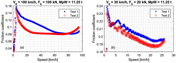
In order to give an example of experimental dispersion, Fig. (1) shows two examples of variation of friction coefficient as a function of speed, for a test of stop-braking, for two different loading conditions: initial speed V0 of 100 km/h, normal force Fk of 100 kN for (a) and V0=30 km/h and Fk=20 kN for (b). Both in (a) and in (b) there are two series of points which represent two repetitions of the same nominal condition. A careful watching of Fig. (1) shows that an acceptable recording of a braking test starts at a speed lower than nominal starting speed and finishes before than 0 km/h, because at the beginning of the braking the applied normal force is not at the designated level and because at low speed torque measurement can be inaccurate. This is the reason why there are no experimental points in the whole interval of variation of the results, from 100 to 0 (a) and from 30 to 0 (b).
In order to fit experimental data by means of polynomial laws, two methods are proposed here: the first employs a fitting polynomial law independent of the starting speed and it is valid in the field [0-120] km/h; the second employs a different fitting polynomial law for each different starting speed (V0) and it is valid in the field [0-V0]. In this method, current speed plays the role of independent variable and friction coefficient of the dependent one; parameters of the fitting polynomial laws are the loading conditions and the normal force between wheel and shoe. Hence, the complete experimental test campaign is described in the first method (method 1) by means of 6 fitting polynomial laws (two levels of mass per wheel and three levels of normal forces) and in the second method (method 2) by means of 24 fitting polynomial laws (levels of method 1 have to be multiplied by four different initial speeds).
In both methods, because of different data dispersion with the speed, a weighted polynomial fitting is employed. The chosen weight w is given by the reciprocal of variance (var) dispersion: i.e.
 Moreover, in order to increase the accuracy of the fitting, a centering and a scaling of data are performed: if v is the speed and respectively µ and s are the mean and standard deviation of data, polynomial coefficients are computed in terms of

In both methods, friction coefficient values for different levels of mass per wheel and of normal forces are computed by means of a linear interpolation. Moreover, if method 2 is used, values of friction coefficient for current speeds outside the field of application of the polynomial laws are computed by means of extrapolation, as described later on.
2.1. Method 1
In this method, for each loading condition and each level of normal force between wheel and shoe, there is only one fitting polynomial law that describes the friction coefficient evolution with the speed. Coefficients are reported in Table (1): first column reports the values of normal force between wheel and shoe in kN; first three rows refer to empty condition (i.e. mass per wheel is 2.5 tons) and last three rows refer to laden conditions (i.e. mass per wheel is 11.25 tons). Polynomial coefficients are from the higher degree to the lower degree. Mean values and standard deviations, in km/h, for all polynomials are 60 and 35.074, respectively.
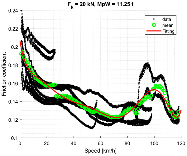
Fig. (2) shows an example of polynomial fitting by means of method 1; fitted curve is reported in solid red, whereas green circles represent average data and black asterisks raw data. Fitting refers to a mass per wheel (MpW) of 11.25 tons and a normal force (Fk) of 20 kN.
For method 1, the speed range always goes from 0 to 120 km/h and Table (1) provides the polynomial coefficients to be used considering a scaled and centred speed as: .
| Fk | Coefficients | |||||||||
|---|---|---|---|---|---|---|---|---|---|---|
| 12 | 3,139e-4 | -4,330e-4 | -1,600e-3 | 4,583e-3 | -2,688e-3 | -1,129e-2 | 1,740e-2 | 1,714e-2 | -3,928e-2 | 1,563e-1 |
| 16 | -2,251e-3 | -4,799e-3 | 1,825e-2 | 2,615e-2 | -5,071e-2 | -4,203e-2 | 5,835e-2 | 3,634e-2 | -5,253e-2 | 1,473e-1 |
| 20 | -2,567e-3 | -3,176e-3 | 1,824e-2 | 1,719e-2 | -4,263e-2 | -2,491e-2 | 4,476e-2 | 2,675e-2 | -5,222e-2 | 1,398e-1 |
| 20 | -4,175e-4 | 7,251e-3 | 7,889e-3 | -3,684e-2 | -3,748e-2 | 4,921e-2 | 5,349e-2 | 3,589e-3 | -2,467e-2 | 1,280e-1 |
| 60 | 6,228e-4 | 4,939e-6 | -3,057e-3 | 1,110e-5 | -2,713e-3 | -1,406e-3 | 1,336e-2 | 2,063e-2 | -3,016e-2 | 1,003e-1 |
| 100 | 1,168e-3 | 2,425e-4 | -5,689e-3 | -9,027e-4 | -5,823e-3 | -4,408e-3 | 3,677e-2 | 3,085e-2 | -2,937e-2 | 9,183e-2 |
2.2. Method 2
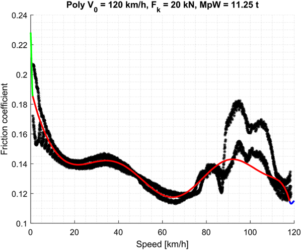
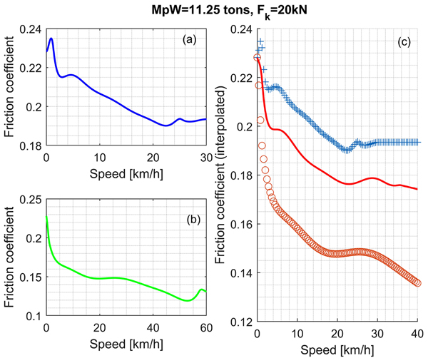
This method is similar to the previous one, except that it requires a different polynomial law for each different starting speed. As an example, Fig. (3) shows the evolution of instantaneous friction coefficient with speed, when V0=120 km/h, Fk=20 kN and MpW=11.25 tons: because of weighted polynomial fitting, fitting curve is close to data from, roughly, 85 km/h to low speed and it is less close to data for high speed, where data dispersion is high (for this test). In this figure, besides experimental data (given by black asterisk), there are three solid lines: 1) red solid line represents the polynomial fitting of data; 2) green solid line represents the connecting third order polynomial to zero speed; 3) blue solid line represents the connecting third order polynomial to maximum (starting) speed. For this method, the speed range, used for braking computations, changes according to the initial speed, i.e. it is not fixed. Firstly, a series of polynomials for speed ranges from 0 to 30, 60, 100, 120 km/h have to be computed and then a linear interpolation is employed, as described in the comment of (Fig. 4).
From the test results obtained for each UIC approved friction material the static friction coefficient is a function of normal force between wheel and shoe; it varies from 0.23 (low normal force) to 0.21 (high normal force). In this paper, variation of friction coefficient between these two bounds is assumed linear with normal force, varying from 12 kN up to 100 kN. Connecting polynomial at low speed is of third order and it guarantees point and slope continuity with polynomial data fitting (red curve). Such third order polynomial has a slope at zero speed given by the straight line that connects static friction coefficient to first point of polynomial data fitting. Different conditions are set for the connecting polynomial at high speed (blue line): this is still a third order polynomial with point and slope continuity with polynomial data fitting, but it has zero slope at maximum (starting) speed V0 and the value of friction coefficient at this speed is equal to the value of friction coefficient at maximum speed of polynomial data fitting.
Polynomial coefficients are reported in Table (2); first 12 rows refer to MpW=2.5 tons the other rows to MpW=11.25 tons. Normal forces for low mass per wheel are 12, 16 and 20 kN; for high mass per wheel they are 20, 60 and 100 kN. First three rows refer to the speed of 30 km/h and normal forces are, respectively, 12, 16 and 20 kN; the next three rows refer to the speed of 60 km/h (with values of normal force as before) and so on.
| Coefficients | |||||||||
|---|---|---|---|---|---|---|---|---|---|
| 0 | -1,104e-3 | 2,080e-3 | 2,923e-3 | -6,806e-3 | -1,003e-3 | 5,575e-3 | -1,737e-3 | -3,050e-3 | 2,386e-1 |
| 0 | 0 | 0 | 0 | 9,825e-4 | 9,291e-5 | -2,307e-3 | -5,376e-4 | -1,425e-3 | 2,494e-1 |
| 0 | 0 | 0 | 0 | 0 | -3,794e-4 | -4,113e-5 | 1,084e-3 | -1,818e-3 | 2,483e-1 |
| -1,276e-6 | 5,872e-4 | -4,169e-4 | -2,985e-3 | 2,583e-3 | 5,073e-3 | -4,399e-3 | 2,698e-3 | -1,344e-2 | 1,955e-1 |
| 0 | 0 | 0 | 0 | 6,229e-4 | 7,419e-5 | -2,662e-3 | 4,918e-3 | -1,304e-2 | 2,011e-1 |
| -8,748e-4 | 8,681e-4 | 4,523e-3 | -4,363e-3 | -6,387e-3 | 5,635e-3 | 4,477e-4 | 3,413e-3 | -1,228e-2 | 2,007e-1 |
| 1,049e-6 | -3,928e-7 | 1,567e-3 | -8,675e-4 | -8,208e-3 | 1,069e-2 | 1,177e-2 | -1,733e-2 | -2,605e-2 | 1,749e-1 |
| -7,828e-4 | 1,530e-4 | 5,550e-3 | -1,417e-3 | -1,496e-2 | 9,298e-3 | 1,760e-2 | -1,336e-2 | -3,100e-2 | 1,686e-1 |
| 1,858e-3 | -2,578e-3 | -8,495e-3 | 1,276e-2 | 8,519e-3 | -1,417e-2 | 5,133e-3 | 2,761e-3 | -3,620e-2 | 1,673e-1 |
| -7,022e-4 | 9,871e-5 | 7,263e-3 | 1,097e-3 | -2,831e-2 | -1,551e-3 | 4,482e-2 | 2,676e-3 | -4,071e-2 | 1,551e-1 |
| -1,337e-3 | 1,745e-4 | 9,875e-3 | 4,453e-4 | -2,838e-2 | -1,331e-4 | 3,639e-2 | 7,852e-3 | -4,053e-2 | 1,470e-1 |
| 0 | 0 | 1,940e-3 | 2,178e-4 | -1,273e-2 | 2,138e-3 | 2,580e-2 | 5,590e-3 | -3,883e-2 | 1,323e-1 |
| -3,515e-3 | 2,079e-3 | 1,648e-2 | -8,651e-3 | -2,335e-2 | 1,119e-2 | 1,133e-2 | -3,345e-3 | -1,285e-2 | 2,017e-1 |
| 5,079e-3 | 1,655e-3 | -2,513e-2 | -4,168e-3 | 4,145e-2 | 6,210e-4 | -2,542e-2 | 3,596e-3 | -2,937e-3 | 1,921e-1 |
| 2,030e-3 | -4,700e-4 | -5,045e-3 | -5,919e-3 | 4,173e-3 | 1,835e-2 | -5,440e-3 | -6,199e-3 | -9,947e-3 | 1,949e-1 |
| -2,255e-3 | 3,377e-3 | 1,377e-2 | -1,637e-2 | -2,628e-2 | 2,970e-2 | 1,317e-2 | -2,347e-2 | -1,152e-2 | 1,472e-1 |
| -2,493e-3 | 1,741e-3 | 1,486e-2 | -7,889e-3 | -2,985e-2 | 1,395e-2 | 2,043e-2 | 4,966e-3 | -2,977e-2 | 1,166e-1 |
| 1,663e-3 | 2,108e-4 | -1,279e-2 | 2,401e-3 | 3,177e-2 | -1,023e-2 | -3,346e-2 | 2,436e-2 | -1,204e-3 | 9,963e-2 |
| 1,384e-3 | -9,101e-6 | -7,037e-3 | -6,732e-4 | 6,073e-3 | 8,897e-3 | 6,974e-3 | -1,290e-2 | -1,955e-2 | 1,435e-1 |
| 7,505e-4 | -1,456e-3 | -2,868e-3 | 5,587e-3 | 1,482e-3 | -8,438e-4 | 1,806e-3 | 4,710e-3 | -2,556e-2 | 1,043e-1 |
| -2,796e-4 | 5,956e-4 | 9,534e-4 | -1,459e-3 | -2,020e-3 | 2,464e-3 | 2,935e-3 | 2,879e-3 | -1,287e-2 | 8,782e-2 |
| -3,474e-3 | -4,719e-3 | 2,524e-2 | 3,382e-2 | -6,988e-2 | -7,914e-2 | 7,712e-2 | 7,146e-2 | -2,747e-2 | 1,198e-1 |
| 5,014e-3 | 1,558e-3 | -2,686e-2 | -9,037e-3 | 4,181e-2 | 1,494e-2 | -1,750e-2 | 9,608e-3 | -2,908e-2 | 1,080e-1 |
| -3,801e-3 | 1,633e-3 | 2,263e-2 | -1,251e-2 | -5,022e-2 | 2,592e-2 | 5,224e-2 | 5,002e-3 | -3,551e-2 | 1,058e-1 |
In this case, also, independent variable, speed, has been centered and scaled; Table (3). reports the value of mean and standard deviation to be used with coefficients of Tables (2 and 3) reports also the field of validity of polynomials reported in (Table 2).
| MpW = 2.5 tons | MpW = 11,25 | ||||||
|---|---|---|---|---|---|---|---|
| Vmin | Vmax | µ | σ | Vmin | Vmax | µ | σ |
| 9,864 | 19,86 | 14,56 | 3,474 | 1,296 | 25,30 | 13,48 | 7,584 |
| 9,648 | 17,65 | 13,53 | 2,868 | 4,032 | 19,03 | 11,94 | 4,955 |
| 9,288 | 14,29 | 11,94 | 1,939 | 6,768 | 16,77 | 11,54 | 3,472 |
| 8,424 | 50,42 | 29,50 | 12,81 | 1,224 | 57,22 | 29,49 | 16,86 |
| 7,488 | 49,49 | 28,50 | 12,81 | 4,752 | 51,75 | 28,01 | 14,25 |
| 5,760 | 46,76 | 26,01 | 12,52 | 7,128 | 52,13 | 29,98 | 13,68 |
| 3,816 | 91,82 | 47,51 | 26,11 | 1,296 | 97,30 | 49,50 | 28,42 |
| 5,400 | 86,40 | 46,00 | 24,08 | 5,400 | 94,40 | 50,00 | 26,39 |
| 6,264 | 88,26 | 47,49 | 24,37 | 4,752 | 94,75 | 49,51 | 26,68 |
| 4,176 | 111,2 | 57,99 | 31,59 | 0,936 | 117,9 | 59,01 | 34,48 |
| 6,408 | 109,4 | 58,00 | 30,44 | 4,104 | 116,1 | 60,49 | 33,04 |
| 8,640 | 105,6 | 57,00 | 28,71 | 6,336 | 114,3 | 60,50 | 31,88 |
Tables (2 and 3). have to be used to compute friction coefficient for intermediate speeds; for low and high speeds, i.e. for connecting polynomials to zero and maximum (nominal) speed of the test, respectively, (Table 4) has to be used.
| Coefficients, for low speed | µ | σ | Coefficients for high speed | µ | σ | ||||||
|---|---|---|---|---|---|---|---|---|---|---|---|
| 1,736e-3 | -2,728e-4 | -4,212e-5 | 2,366e-1 | 4,988 | 3,296 | -1,132e-3 | 1,993e-3 | 2,010e-3 | 2,288e-1 | 24,572 | 3,493 |
| 1,501e-3 | -3,515e-3 | 4,144e-3 | 2,488e-1 | 4,968 | 3,265 | 7,523e-4 | -1,283e-3 | -1,537e-3 | 2,485e-1 | 23,546 | 4,109 |
| 9,562e-4 | -4,582e-3 | 5,269e-3 | 2,505e-1 | 4,935 | 3,215 | -5,473e-4 | 8,978e-4 | 1,295e-3 | 2,447e-1 | 22,017 | 5,022 |
| -1,124e-3 | -3,424e-3 | 4,087e-3 | 2,401e-1 | 4,442 | 2,937 | 6,487e-4 | -1,058e-3 | -1,297e-3 | 1,899e-1 | 55,039 | 3,255 |
| -4,299e-4 | -3,087e-3 | 4,486e-3 | 2,412e-1 | 3,943 | 2,649 | 1,694e-4 | -2,807e-4 | -3,429e-4 | 1,897e-1 | 54,541 | 3,540 |
| -1,028e-3 | -2,494e-3 | 4,107e-3 | 2,360e-1 | 2,966 | 2,106 | -6,363e-4 | 1,103e-3 | 1,292e-3 | 1,839e-1 | 53,051 | 4,391 |
| -7,447e-4 | -9,776e-4 | 9,290e-4 | 2,312e-1 | 1,963 | 1,524 | 1,044e-3 | -1,824e-3 | -1,705e-3 | 1,575e-1 | 95,582 | 2,901 |
| -1,405e-3 | -1,882e-3 | 1,019e-3 | 2,303e-1 | 2,914 | 2,029 | 2,491e-4 | -4,118e-4 | -5,563e-4 | 1,410e-1 | 93,027 | 4,428 |
| 1,397e-3 | 2,141e-3 | -1,590e-3 | 2,257e-1 | 3,408 | 2,309 | 9,187e-4 | -1,476e-3 | -2,039e-3 | 1,431e-1 | 94,020 | 3,861 |
| -1,090e-3 | -8,259e-4 | -2,491e-3 | 2,250e-1 | 2,363 | 1,670 | 5,664e-4 | -8,732e-4 | -1,186e-3 | 1,479e-1 | 115,518 | 2,999 |
| -1,869e-3 | -4,483e-3 | 5,566e-3 | 2,410e-1 | 3,426 | 2,335 | 5,190e-4 | -8,486e-4 | -1,077e-3 | 1,465e-1 | 114,534 | 3,550 |
| -1,907e-3 | 1,064e-3 | -1,926e-3 | 2,164e-1 | 4,464 | 2,970 | 1,027e-3 | -1,754e-3 | -2,202e-3 | 1,345e-1 | 112,540 | 4,696 |
| -5,386e-3 | -7,751e-3 | 3,777e-3 | 2,346e-1 | 0,765 | 0,679 | -4,705e-4 | 6,944e-4 | 7,365e-4 | 1,924e-1 | 27,549 | 1,794 |
| 3,248e-3 | 7,251e-3 | -7,582e-3 | 2,030e-1 | 2,339 | 1,640 | 2,584e-3 | -3,964e-3 | -5,964e-3 | 1,936e-1 | 24,503 | 3,601 |
| 5,863e-3 | 6,901e-3 | -7,151e-3 | 2,029e-1 | 3,471 | 2,403 | 3,045e-3 | -5,282e-3 | -6,168e-3 | 1,956e-1 | 23,051 | 4,390 |
| 4,629e-3 | 3,521e-3 | -2,255e-2 | 2,048e-1 | 0,741 | 0,652 | 1,415e-3 | -1,825e-3 | -1,713e-3 | 1,333e-1 | 58,556 | 1,206 |
| -4,186e-3 | -6,086e-3 | 6,729e-3 | 2,290e-1 | 2,459 | 1,806 | 1,181e-3 | -2,040e-3 | -1,988e-3 | 1,207e-1 | 55,575 | 2,911 |
| -6,018e-3 | -7,190e-3 | 3,846e-3 | 2,115e-1 | 3,903 | 2,591 | 8,494e-4 | -1,278e-3 | -1,739e-3 | 1,126e-1 | 56,014 | 2,715 |
| 4,582e-3 | 4,325e-3 | -1,749e-2 | 2,095e-1 | 0,765 | 0,679 | 2,696e-4 | -3,596e-4 | -3,120e-4 | 1,260e-1 | 98,574 | 1,180 |
| 2,600e-4 | 5,135e-3 | -1,155e-2 | 1,927e-1 | 2,914 | 2,029 | 3,731e-4 | -5,816e-4 | -6,070e-4 | 1,023e-1 | 97,057 | 2,071 |
| -1,251e-3 | 5,341e-3 | -2,070e-2 | 1,688e-1 | 2,459 | 1,806 | 4,650e-4 | -7,978e-4 | -6,121e-4 | 9,384e-2 | 97,107 | 1,999 |
| 1,829e-2 | 5,708e-3 | -3,936e-2 | 2,040e-1 | 0,468 | 0,662 | -1,194e-3 | 2,124e-3 | 5,252e-4 | 1,132e-1 | 118,734 | 0,975 |
| 1,433e-3 | 4,604e-3 | -8,452e-3 | 2,019e-1 | 2,351 | 1,655 | 1,429e-3 | -1,884e-3 | -2,187e-3 | 1,008e-1 | 118,021 | 1,549 |
| -2,680e-3 | -5,337e-4 | -3,259e-3 | 1,978e-1 | 3,417 | 2,322 | -1,979e-3 | 3,029e-3 | 3,322e-3 | 1,069e-1 | 117,048 | 2,085 |
If method 2 is used to compute friction coefficient and train starting speed is different from the experimental ones (i.e. 30, 60, 100 and 120 km/h), a (linear) interpolation of data is required.
Fig. (4) shows an example that refers to a starting speed of 40 km/h, when the MpW=11.25 tons and Fk=20 kN: as it is clear, the curve that refers to the lower starting speed is linearly extrapolated and then the linear interpolation is applied. Fig. (4c) shows with solid line the interpolating polynomial that describes the instantaneous friction evolution with speed for a stop – braking from initial speed of 40 km/h.
However, effective use of the model requires further interpolations for values of mass per wheel and normal forces between wheel and shoe that are different from the test conditions. Results reported in this paper employ linear interpolations also to manage such situations.
From the above description, method 2 is more complex to handle than method 1.
3. MATCHING AGAINST EXPERIMENTAL TESTS
Polynomial fitting reported above has been tested against experimental data provided by TRENITALIA. Such experimental data refer to slip tests performed on two wagons: Eanos, equipped with a classical empty/load braking device, and Sgns, equipped with a more recent auto-continuous braking device. It is here recalled that:
- empty/load braking systems have two levels of braked weight, one for empty (low payload) conditions and another for laden conditions. They have also a level of mass (called “inversion mass”) to switch from one condition to another. Maximum air pressure in brake cylinder is around 1.2 bar in empty condition and 3.8 bar in laden condition.
- Auto-continuous braking systems have the characteristic to change wagon braked-weight with wagon mass, continuously. For this type of Sgns wagon, air pressure in brake cylinder is 3.8 bar and braking force is changed by mechanically varying rigging ratio.
Table (5) reports the stopping distances computed numerically, by method 1 and 2, and measured experimentally, for above types of wagon in different loading conditions and with different starting speeds (V0).
Error with respect to experimental measurements is always below 5% and method 2 is usually closer to experimental measurements than method 1: this means that more complexity of method 2 provides a better accuracy. This error has the same order of magnitude of error obtained by TrainDy [14], during its validation process, when cast iron brake shoes were tested and Karwatzki analytical law [17] was employed. Moreover, experimental values reported in Table (5) are the result of a correction operated according to UIC CODE 544-1, Appendix F.3 [18]. In fact, actual initial speed is usually different from the nominal starting speed; hence, as Table (6) shows, from measured values (label “Measured SD”), s_cor1 values are computed. From their mean value (s_cor1 av.) another correction is applied, considering the current rigging efficiency and the time to reach the maximum pressure in brake cylinder (BC), getting the value s_cor2. Comparing data of Table (6) with data of Table (5), stopping distances computed by method 2 provide an error of the same order of magnitude as the experimental tests.
| Eanos | ||||
|---|---|---|---|---|
| V0 [km/h] | Method 1 [m] | Method 2 [m] | Exp [m] | |
| Empty | 100 | 443.46 | 423.20 | 420.64 |
| Laden | 100 | 596.21 | 607.21 | 596.22 |
| Empty | 120 | 641.41 | 639.54 | 634.70 |
| Sgns | ||||
| Empty | 100 | 486.00 | 455.26 | 457.25 |
| Laden | 100 | 566.12 | 571.80 | 586.11 |
| Empty | 120 | 723.27 | 708.94 | 690.34 |
| #Test | Measured SD [m] | s_cor1 [m] | s_cor1 av. [m] | s_cor2 [m] |
|---|---|---|---|---|
| 7 | 374.05 | 361.93 | 371.66 | 420.64 |
| 9 | 370.66 | 365.96 | ||
| 10 | 383.88 | 366.03 | ||
| 11 | 381.12 | 383.34 | ||
| 17 | 390.62 | 382.54 | ||
| 19 | 353.39 | 370.15 |
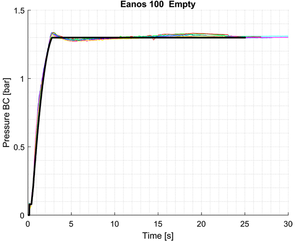
Fig. (5) shows the time evolution of air pressure in BC for Eanos wagon. Test considered is emergency braking in empty conditions from nominal speed of 100 km/h. Numerical results are displayed by black solid line, experimental results by coloured solid lines. Experimental results and numerical results are in a good agreement; anyway, experimental results show an oscillation of air pressure, which is not displayed by numerical results. The reason of such difference is that air pressure in BC is computed numerically by means of a stationary model from limiting curves and transfer function of distributor [19]. This (small) difference between numerical and experimental pressure in BC differentiates numerical and experimental results in terms of speed and acceleration. It is worth remembering, in fact, that the deceleration of the wagon is the effect, among other aspects, of the product between the normal force between shoes and wheel and the coefficient of friction. Friction coefficient depends not only on the speed of the rolling stock but also on the value of the normal force between wheel and shoe, which depends, among other aspects, on the value of the air pressure in the brake cylinder.
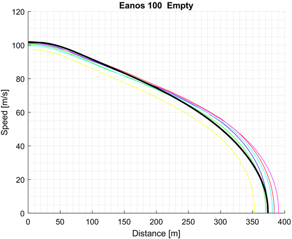
Similarly, Fig. (6) shows, for the same experimental conditions of Fig. (5), the evolution of speed with position on the track measured experimentally (coloured curves) and computed numerically (black curve). The numerical result of Fig. (6) refers to a starting speed equal to test #7 of Table (6) and to other influencing parameters (e.g. rigging efficiency, time to reach maximum pressure in BC, and so on) that match this experimental test.
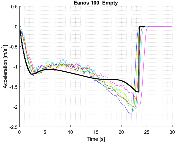
Fig. (7) displays the acceleration in the same numerical conditions used for Fig. (6). Experimental data have been filtered by applying a spline to speed data with a sampling frequency of 10 Hz (original data have a sampling frequency of 5 kHz). This result shows the worst agreement in comparison with experimental data. The difference in terms of maximum acceleration (since it is negative it is actually a deceleration) is up to 20%. However, since the wagon is a freight wagon, this error has not a big importance, moreover, since it occurs at almost zero speed, it has usually low importance for derailment risk (when high compressive in-train forces govern this type of accident).
Similar results are also obtained for the other test conditions, both for Eanos wagon and Sgns wagon, and are not shown here for the sake of conciseness.
4. EFFECT ON IN-TRAIN FORCES
Aiming to provide a first understanding of the effect of CBB type LL on in-train forces, a series of simulations on homogeneous trains have been performed. An emergency braking on a straight plain track from 30 km/h has been simulated, considering trains whose mass is equal to the current limits allowed by UIC CODE 421 [10] for different braking regimes (P, GP). Table (7) shows simulations results in terms of stopping distance, 10 m Longitudinal Compressive Force (LCF10) and instantaneous Longitudinal Tensile Force (LTF). LCF10 is the minimum in-train compressive force acting in the 10 m before the current position. LCF10 is used to synthetically test the safety against derailment of train makeup, whereas LTF can be used to evaluate the risk of train disruption. In-train compressive forces are displayed with a negative sign. According to the simulations, CBB type LL effect in-train forces providing lower values for G and P regimes and higher values for GP and LL regimes. Best performances are for P regime where both stopping distance and in-train forces are usually reduced (in absolute value).
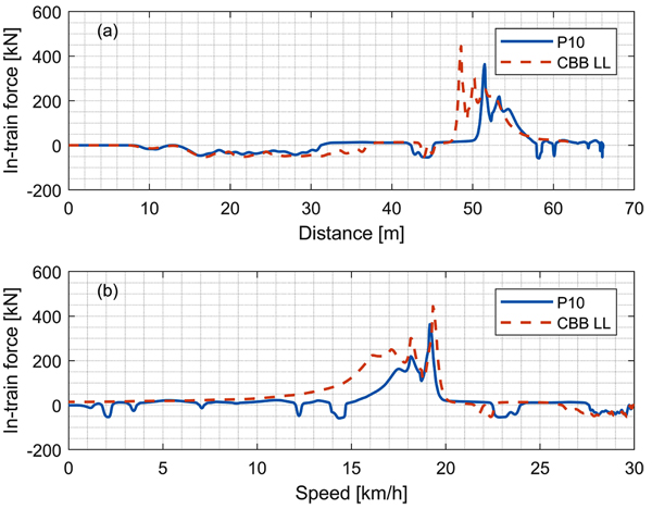
Finally, Fig. (8) shows the evolution of maximum in-train tension force for homogeneous trains equipped with Eanos wagons performing an emergency braking from 30 km/h, in braking regime LL. Maximum values of instantaneous longitudinal tension forces occur at similar speeds and far from low speeds where acceleration peaks have been experienced.
CONCLUSION
Noise of rail freight transport is becoming an important issue for Railway Undertakings in recent years. The use of Composite Brake Blocks (CBB) is a contribution to solve this problem, replacing the “historical” cast iron (P10). Among the types of CBB, the one that allows a quicker use is the “LL type”. Braking performance of this friction material is accurately measured by bench tests; then it is further verified by means of individual wagon slip and in-service tests.
This paper illustrates two methods by which computing of a series of polynomial curves from the experimental data on the bench can be performed: the first computes polynomial law from maximum speed (120 km/h) to zero, whereas the second computes several polynomials for different initial starting speeds. These curves describe the trend of friction coefficient as a function of speed for different wagon mass and the intensity of braking action. The proposed model is verified by means of a comparison with slip tests of two Trenitalia freight wagons, obtaining satisfactory results in terms of stopping distances, speed and acceleration. Validation results show that second method is usually more accurate than the first method. The maximum error against experimental data is experienced in acceleration peak, where an error of 20% is found for the second method. However, this error occurs almost at zero speed where inaccuracies do not have an important effect on stopping distance or on in-train compressive forces. Numerical results here reported show that high in-train tension forces occur at speed far from zero.
This work is the first one in which certified experimental data are used to derive a numerical model of the instantaneous coefficient of friction for these CBB. This allows the computation of Longitudinal Train Dynamics for trainsets where wagons equipped with CBB type LL are employed; these new types of trainsets are going to replace the current trains operated by European Railway Undertakings. By polynomial data here reported, computation of in-train forces of these trainsets is made available to all the researchers in this field. Moreover, since the paper shows some differences in terms of in-train forces, see (Table 7 and Fig. 8), it is important to further investigate this topic, for example by means of statistical studies, in order to verify if new trainsets have the same level of safety of the previous ones, with respect to longitudinal dynamics.
| Wagon | Stopping Distance [m] | LCF10 [kN] | LTF [kN] | ||||
|---|---|---|---|---|---|---|---|
| P10 | LL | P10 | LL | P10 | LL | ||
| 800 tons in P | Eanos | 56.44 | 51.01 | -8.862 | -7.874 | 78.63 | 68.47 |
| Sgns | 58.19 | 53.29 | -21.12 | -23.49 | 80.43 | 72.74 | |
| 1200 tons in GP | Eanos | 58.42 | 52.72 | -52.85 | -59.54 | 97.52 | 109.3 |
| Sgns | 60.10 | 54.97 | -31.94 | -50.85 | 102.7 | 130.4 | |
| 1600 tons in LL | Eanos | 66.11 | 61.96 | -55.70 | -64.51 | 363.4 | 444.5 |
| Sgns | 66.83 | 62.63 | -24.31 | -27.35 | 281.4 | 444.3 | |
| 2500 tons in G | Eanos | 88.35 | 92.31 | -80.86 | -75.26 | 102.4 | 53.73 |
| Sgns | 90.91 | 95.81 | -77.93 | -68.85 | 115.2 | 83.96 | |
APPENDIX: SHOE GEOMETRY
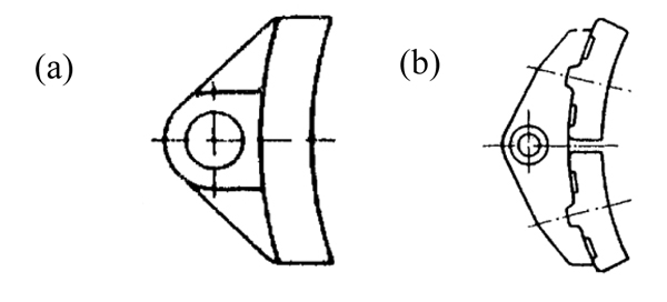
Reference [20] mentions two types of shoes “Bg” and “Bgu”. According to International Union of Railways (UIC), Bg stands for “Bremse sohle geteilt”, brake shoe split, whereas Bgu stands for “Bremse geteilt mit unterteilter Sohle”, brake shared with subdivided shoe. If the wheel is pressed by two shoes of type Bg or Bgu, the labels 2xBg and 2xBgu are used, respectively.
Fig. (9) shows braking scheme of a wagon equipped with an empty-load device: dimensions here reported are in millimeters and represent an example of geometry. A configuration 2xBg is displayed in this figure. Fig. (10) shows more in detail the geometry of Bg shoe (a) and Bgu shoe (b). Dimensions of friction surfaces for these two types of shoes are as follows (in millimeters): 320x80, for Bg and two surfaces of 250x80, for Bgu.

CONSENT FOR PUBLICATION
Not applicable.
CONFLICT OF INTEREST
The authors declare no conflict of interest, financial or otherwise.
ACKNOWLEDGEMENTS
Declared none.

