All published articles of this journal are available on ScienceDirect.

Travel-time Prediction Using K-nearest Neighbor Method with Distance Metric of Correlation Coefficient
Abstract
Background:
Real-time Travel Time (TT) information has become an essential component of daily life in modern society. With reliable TT information, road users can increase their productivity by choosing less congested routes or adjusting their trip schedules. Drivers normally prefer departure time-based TT, but most agencies in Korea still provide arrival time-based TT with probe data from Dedicated Short-Range Communications (DSRC) scanners due to a lack of robust prediction techniques. Recently, interest has focused on the conventional k-nearest neighbor (k-NN) method that uses the Euclidean distance for real-time TT prediction. However, conventional k-NN still shows some deficiencies under certain conditions.
Methods:
This article identifies the cases where conventional k-NN has shortcomings and proposes an improved k-NN method that employs a correlation coefficient as a measure of distance and applies a regression equation to compensate for the difference between current and historical TT.
Results:
The superiority of the suggested method over conventional k-NN was verified using DSRC probe data gathered on a signalized suburban arterial in Korea, resulting in a decrease in TT prediction error of 3.7 percent points on average. Performance during transition periods where TTs are falling immediately after rising exhibited statistically significant differences by paired t-tests at a significance level of 0.05, yielding p-values of 0.03 and 0.003 for two-day data.
Conclusion:
The method presented in this study can enhance the accuracy of real-time TT information and consequently improve the productivity of road users.
1. INTRODUCTION
Real-time Travel Time (TT) information has become an essential part of modern society. It can reduce road users’ travel times by choosing a less congested route or rescheduling their trip plans to nonpeak hours. Traditionally, TTs were collected using vehicle detectors that use different sensors, such as loop, video image, microwave, ultrasonic. However, as wireless communication technologies evolve, probe-base systems such as GPS, Dedicated Short-Range Communications (DSRC), and Bluetooth/Wi-Fi are attracting more interest in developed countries. These wireless technologies have two main merits: efficiency for deployment and maintenance, and their ability to obtain direct link TT. Compared to vehicle detector-based TT collection systems, DSRC-based systems are known to be more affordable so DSRC scanners are broadly installed on many roadways by many road agencies in Korea. Using traffic data from vehicle detectors, link TTs should be estimated with the assumption of homogeneity of TTs in the segment covered by a detector. However, this assumption is frequently violated on the signalized arterials that this study focuses on. In Korea, an Electronic Toll Collection System (ETCS) is already based on 5.8 GHz DSRC technology, indicating that agencies could simply install DSRC scanners on the road to collect DSRC-equipped probe data. As of 2017, more than 20% of vehicles on the road could be used as probes with DSRC scanners. The penetration rate was similar in 2013 when the data were gathered for this study. Of course, standard measures for protecting drivers’ privacy are applied to DSRC TT systems not only by encrypting user identifications, but also by discarding individual probe data after generating link TTs. However, probe TTs obtained using DSRC scanners inevitably include time lags equivalent to the TTs experienced by the probes on the segment because TTs, which normally called arrival time-base travel times, are calculated after probe vehicles complete the trip. Therefore, TT prediction is more emphasized in probe-based real-time TT provision systems than detector-based TT provision systems.
Several prediction techniques have been applied to real-time TT information systems. Among the most popular techniques are the Kalman Filter (KF), Artificial Neural Network (ANN), time series analysis (TSA), and the k-Nearest Neighbor (k-NN) method. KF, named after R. E. Kalman, one of the primary developers of its theory, is an algorithm that uses time series measurements and produces estimates of unknown variables [1]. The algorithm is recursive, using a two-step process. In the prediction step, it generates estimates of the current state variables, which include uncertainties. In the second step, when the next measurement is obtained, these estimates are updated using a weighted average. In this case, less weight is assigned to the estimates with higher uncertainty [2]. Since it only uses the current input measurements and previously estimated state along with its uncertainty matrix, its implementation is quite simple. In contrast, other techniques listed above require a large amount of high quality historical TTs. However, KF can only predict TTs one step ahead even though road users normally want to know TTs several steps ahead (or departure time-based TTs: the travel times to be experienced by vehicles that are departing the start point after receiving TT information). ANN is a computing system inspired by the biological neural networks that organize animal brains, learning from archived data to perform a certain task [3]. Among many ANN algorithms, time-delay neural networks that recognize features in sequential data are regarded as an optimal solution for predicting traffic data, which, reflecting people’s daily activities, normally shows repetitive day-to-day patterns [4]. TSA is a methodology for interpreting data in a time sequence to predict future values using previously observed values [5]. Autoregressive, integrated, and moving average models are three general classes for modeling variations in time sequential observations. Combinations of the three models produce Autoregressive Integrated Moving Average (ARIMA) models that were proven appropriate for predicting traffic data [6]. However, both ANN and TSA are notorious for their lack of universality (or transferability), indicating that if new TT patterns deviate from TT patterns used for training, performance could deteriorate significantly. In reality, changes in TT patterns frequently occur due to local events, traffic accidents, weather, roadwork, and other difficult to predict phenomena. Hence, although based on a sophisticated theoretical background, real-world systems using ANN and TSA to predict TTs are hardly observed. k-NN is a nonparametric method applied for classification or regression. In both cases, the input variables are the k closest learning examples in the feature space [7]. The method is useful because it assigns more weight to nearer neighbors by measuring the distance between current and historical values [8]. A commonly used distance metric is the Euclidean distance. From the perspective of TT prediction, k-NN has advantages over KF, ANN, and TSA. It can not only predict TTs multiple steps ahead (or departure time-based TTs), but it can also recursively include newly collected TTs as a training set in order to continuously adjust to new TT patterns over time. For this reason, k-NN is drawing substantial interest from road agencies in Korea. Table 1 summarizes the pros and cons of each technique described above.
| Method | Advantage | Disadvantage |
|---|---|---|
| KF | Do not require large amount of historical data | Impossible to predict multiple-step-ahead travel times |
| ANN and TSA | Sophisticated and accurate | Do not consider changes in travel-time pattern |
| k-NN | Flexible to changes in travel-time pattern | Long time to execute |
Increasing interest in k-NN for real-time TT prediction is not limited to Korea. Studies have also been performed to apply k-NN to predict traffic data worldwide. Myung et al. proposed a TT prediction model based on k-NN using data from vehicle detector systems and automatic toll collection systems deployed on freeways, and demonstrated the superiority of the proposed model over six other models including KF [9]. Qiao et al. applied a set of four prediction models including historical average, ARIMA, KF, and two types of k-NN algorithms to probe TT data from Bluetooth scanners installed on I-66 in Virginia. k-NN models outperformed other techniques by decreasing errors in prediction accuracy by more than 10% throughout the day and by 20% for peak hours [10]. They also applied a new k-NN model for predicting multi-step ahead TT and verified the superiority of the suggested model over ARIMA using both historical and real-time heterogeneous traffic and weather data collected on I-95 in Maryland [11]. Wu et al. compared several TT prediction techniques including k-NN, historical average, and ANN, and demonstrated that the proposed k-NN model that considered both temporal and spatial information significantly improved forecasting accuracy. This was a result of numerical tests using probe data obtained from 180 taxis running in Guiyang, China [12]. Lim et al. predicted departure time-based real-time TT with k-NN, KF, and historical average techniques using arrival time-based probe TT data from DSRC scanners installed on suburban arterials, and demonstrated the superiority of the applied k-NN technique over other techniques [13]. Tak et al. applied a multi-level k-NN algorithm designed for forecasting TT with increased computational efficiency and prediction accuracy. The proposed algorithm consisted of three parts: classification, global matching, and local matching. It showed 5% error range even in congested traffic situations, indicating satisfactory performance compared to existing methods [14]. Yu et al. proposed a short-term traffic condition prediction model based on k-NN. They proposed a multi-step prediction model with consideration of the time-varying and continuous characteristics of traffic flow. Evaluation using GPS data of taxis in Foshan city, China, revealed better performance compared with the support vector machine, ANN, real-time-data model, and history-data model [15]. Zhong et al. investigated the key factors of k-NN through four tests and presented two findings: no linear improvement with increases in data size and enhancement of prediction accuracy with more information included in the state vector [16].
All the previous studies described above used Euclidean distance to find the predefined (k in number) nearest neighbors. However, since the Euclidean distance can only consider the proximity between current and historical values, it potentially shows some deficiencies in TT transition situations, such as increasing TTs followed by decreasing TTs. During the TT transition period, the TT trend along with nearness play an important role in accurate TT prediction. This will be discussed in detail with examples in the following section.
In this study, a correlation coefficient was employed to measure the similarity between current and historical TTs to resolve deficiencies of previous studies. In addition, to compensate for the differences between current and historical TTs, a regression equation was applied to historical TT to obtain the optimal value for a predicted TT. Since correlation coefficients can consider the trend in the current and historical TTs and regression equations can adjust the difference between current and historical TTs, the proposed k-NN method is expected to overcome shortcomings of previous methods. The remainder of this article is structured as follows. In the next section, the traditional k-NN is described in detail and its problems in TT transition situations are described, followed by the description of a new k-NN method that surmounts the problems of the conventional k-NN method. Subsequently, the proposed method is evaluated using 10 experiment cars driven on the segment with 5 minutes headway at the maximum. Finally, the significance of this study will be discussed with a summary and suggestions for future studies.
2. METHODS
2.1. Traditional k-NN Method
Davis and Nihan firstly applied the traditional k-NN method to short-term freeway traffic forecasting [17]. The input variables to constitute the state vector for their model are TTs in the continuously archived previous time intervals. The model searches k-nearest neighbors in the predefined historical records using a combined group (n aggregation intervals) of continuous TTs. The basic assumption behind the method is that the future TTs to be predicted are closely related to the TTs in previous time intervals. This assumption seems to be reasonable in that traffic on the road is generated from human activities that are recursive in nature. The process of the conventional k-NN algorithm can be expressed by equations 1-3 and operates in five steps as follow:
- Construct a historical database. For this study, a month of weekday TTs in 5-min interval were used.
- Select n continuously combined previous intervals. For this study, a 30 minute (or six 5-min intervals) series of data that showed the optimal performance for the conventional k-NN according to a previous study (13) were employed.
- Compute the distance metric defined as the Euclidean distance and select the number of k. For this study, the selected number of k was 4 according to a previous study [15] that demonstrated that k values greater than 4 show little improvement in prediction accuracy. This rule was found to hold for the TT data in this study.
- Determine k-nearest neighbors according to the computed distance metric.
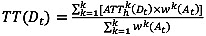
- Forecast the target TT (the departure time-based TT at the same time with the arrival time-based TT) by taking the average of the k-nearest neighbors weighted by the calculated Euclidean distance.
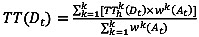
(1) 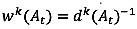
(2) 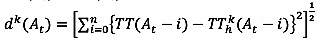
(3)
where TT(Dt) = departure time-based travel time at time t, TThk(Dt)= k-th departure time-based travel time at historical time t, wk(At) = k-th weight of arrival time-based travel time at time t, dk(At) = k-th distance between current and historical arrival time-based travel time at time t, TT(At) = current arrival time-based travel time at time t, TThk(At) = k-th historical arrival time-based travel time at time t, and i= aggregation interval (e.g. 5 min).
2.2. Problems in Traditional k-NN Method
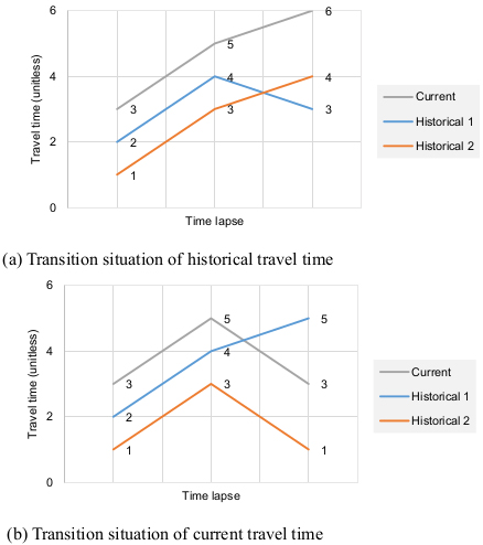
The traditional k-NN method is one of the most widely used nonparametric pattern matching techniques and its robustness has been proven [18-20]. The essence of the nonparametric regression is to find the optimal forecasting values for current observations in the neighborhood in a historical database with similar state vectors. However, as stated earlier, since the traditional k-NN method that uses the Euclidean distance only considers the closeness between the present and the historical observations to find the nearest neighbors, it shows shortcomings in certain situations as exemplified in Fig. (1).
In Fig. (1), one current series and two historical candidate series for the nearest neighbors are plotted. One historical series in (a) and the current series in (b) show trend-changing conditions where values are falling immediately after rising. From the perspective of probe TTs, these changing conditions are normally observed during peak hours. When employing Euclidean distance as a measure of similarity, the predicted values could deviate from the actual observations due to failing to consider the trends. To overcome this problem, a correlation coefficient was used to find historical TTs with the similar trend. A regression equation derived by the ordinary least squares method was then applied to adjust the difference between the current and the historical series. The following section describes the details of the proposed k-NN method.
2.3. Proposed k-NN Method
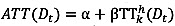
The process of the proposed k-NN in this study is essentially the same with the conventional k-NN method. The only difference is that a correlation coefficient combined with a regression equation is included. To find the optimum value for prediction, the trend as well as the proximity between current and historical series is taken into account. Due to its inability to account for the trend, the traditional k-NN method showed some deficiencies (Fig. 1). On the other hand, since the proposed k-NN method can account for the trend using a correlation coefficient as well as the proximity using a regression equation, it is expected to resolve the shortcomings in traditional k-NN. TT prediction values are obtained by taking the average of the adjusted historical TTs weighted by the correlation coefficients. The proposed k-NN can be expressed in equations 4-6.
 |
(4) |
 |
(5) |
 |
(6) |
where ATThk(Dt) = k-th adjusted departure time-based travel time at historical time t, α and β = intercept and slope of regression line for a set of TT(At-i) and TThk(At-i), and rk(At) = correlation coefficient for each pair of current and k-th historical arrival time-based travel times.
3. EVALUATION
3.1. Data for Evaluation
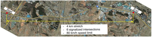
TT data for this study were obtained from the DSRC traffic information system deployed on a signalized arterial in Pyeong Taek region, South Korea (Fig. 2). Traffic on the 4 km stretch of the 4-lane roadway with an 80 km/h speed limit is controlled by six traffic signals. Due to interruptions by the traffic signals, the average travel speed on the stretch under free-flow conditions is approximately 50 km/h.
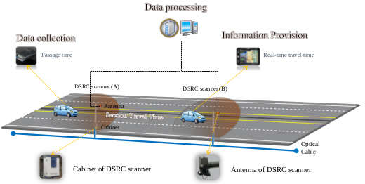
As illustrated in Fig. (3), the DSRC traffic information system consists of a roadside unit (RSE) and an On-Board Unit (OBU). The RSE scans the unique identifications (IDs) of OBU mounted on passing cars. As mentioned above, the original purpose of installing the OBU was for ETCS. Once a car equipped with DSRC OBU passes two consecutive RSEs, a probe TT is generated by matching the unique ID of the OBU. Through the OBUs, real-time TT and incident (accident, lane closure, etc.) information can also be received from the RSEs.
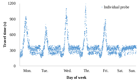
Many outlying observations that deviated significantly from valid observations were gathered. The main reason for outlier occurrence was entry/exit maneuvers and intermittent stops at roadside stores on the corridor. Hence, a robust outlier removal technique developed by Jang [21] for probe TT data on signalized arterials was applied to clean the probe TTs. The applied technique was proven to be superior to other techniques when evaluated with the TT data on the subject segment. Individual probe TTs filtered using this technique for one week (Jan. 21-27, 2013) showed a typical commuter route where morning peak hours (7:00-9:00 a.m.) during weekdays are obvious and no congestion is observed during weekends (Fig. 4). TTs during peak hours on weekdays are 3-4 times longer than those during nonpeak hours. Also, the range of TTs under free-flow conditions is relatively high, possibly due to traffic signals. The significance of real-time TT prediction is highlighted during peak hours because, under noncongested conditions, predicted vs. current TTs do not generally show notable differences. The peak hour (7:00-9:00 a.m.) probe TTs on two weekdays (Feb. 5th-6th, 2013) were therefore considered for the application of the conventional and the proposed k-NN methods. A month-long weekday TTs (January in 2013) on the same stretch were included in the historical database. As shown in Table 2, the average TTs on the two data sets were similar due to the recurrent TT patterns observed on the section during weekdays.
| Item | Historical data set | Prediction data set |
|---|---|---|
| Perioda | Jan. 1st – 30th, 2013 | Feb. 5th – 6th, 2013 |
| Average nonpeak hour travel time | 298 s | 308 s |
| Average peak hour travel timeb | 654 s | 667 s |
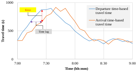
Ten experiment cars were employed to collect ground truth data. The drivers instructed to drive the cars with floating car method which makes the number of cars overtaking the experiment car and overtaken by the experiment car to be equivalent. At least one experiment car was driven within the aggregation interval of 5 minutes. The ground truth TTs were obtained based on the departure time of each experiment car. Fig. (5) shows the comparison between the ground truth TTs and arrival time-based TTs obtained by the DSRC system. The time lag phenomenon is explicitly observed when real-time TT information is provided with arrival time-based TTs, which is the problem with the current practice. As mentioned earlier, in probe-based TT systems, TTs on the corridor can be obtained only after the probes pass the end point. Hence, drivers provided with arrival time-based TT information are frustrated due to the time lags. For this reason, real-time TT predictions should be emphasized to maximize the utility of probe-based TT systems.
3.2. Numerical Analysis
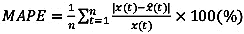
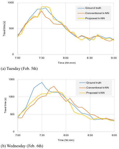
The conventional and proposed k-NN methods were applied to the data described in Table 1 to predict probe TTs on two days. Predicted TTs along with the ground truth data (departure time-based TTs) are plotted in Fig. (6). Compared to Fig. (5), the two methods apparentaly reduced the time lag and therefore increased the accuracy of TT information. However, the prediction methods cannot be easily differentiated. Therefore, predicted TTs were evaluated with an evaluation index of mean absolute percent error (MAPE) as expressed in equation 7, and the results were analyzed for comparison.
 |
(7) |
where MAPE= mean absolute percent error, n= number of samples, x(t)= actual (observed) travel time, and  = predicted travel time.
Table 3 shows a summary of the statistical analyses. Since the proposed k-NN was developed to improve the performance of conventional k-NN in TT transition situations, the results were categorized into two parts: the entire period and the transition period. Considering the daily TT patterns in Fig. (6), the time gap between 7:20 and 8:00 a.m. was arbitrarily selected as the transition period. As investigated in Fig. (1), the traditional k-NN shows deficiencies in trend-changing (or transition) situation so the evaluation period was categorized into two parts-whole and transition period.
Average errors in predicted TTs on the two days were decreased 3.7 percentage point for the whole period and 5.3 percentage point for the transition period when the proposed k-NN method was applied. The differences in prediction errors were also significant according to t-statistics at the 95% confidence interval: the t-statistics for one-tailed tests were higher than the critical t-statistics for all cases except the whole period on Tuesday. The correlation coefficients computed four times for every single TT prediction ranged from 0.61 to 0.99. The slopes and y-intercepts of the regression models ranged from 0.51 to 1.53 and 0 to 388, respectively. All the statistics was statistically significant at 0.05 significance level.
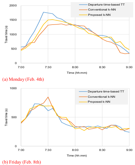
Due to difficulties in gathering ground truth data using experiment cars, the evaluation period was limited to two days. However, considering the similarity of the daily TT patterns plotted in Fig. (4), the consequences in Table 2 can be reasonably accepted. Fig. (7) shows the predicted TTs by the traditional and proposed methods against departure time-based TTs. Although the departure time-based TTs are not ground-truth data, it can reinforce the superiority of the suggested method in that the TTs predicted by the suggested method are closer to the departure time-basd TTs during the transition periods where the proposed method assumed to outperform.
4. DISCUSSION
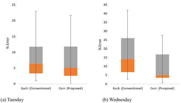
As described above, the newly proposed k-NN method mitigates the time lag phenomenon in the DSRC probe-based TT provision system deployed in signalized arterials in Korea. Error reductions were more prominent in TT transition states where the conventional k-NN showed relatively low performance; this phenomena can be attributed to the fact that, whereas the conventional k-NN only takes closeness into account, the proposed method considers both closeness and trend simultaneously. This outcome satisfies the intention of this study. For Tuesday data, the improvement in the proposed k-NN was minimal over the whole period, but the TT prediction accuracy was significantly enhanced during the transition period. For Wednesday data, improvements during the transition period as well as during the whole period were statistically significant. Furthermore, comparison of the quartiles of the conventional and proposed method where lower values were obtained by the proposed method reinforces the superiority of the proposed method to the convention k-NN (Fig. 8).
| Classification | Statistics | Tuesday (Feb. 5th) | Wednesday (Feb. 6th) | ||
|---|---|---|---|---|---|
| Con. k-NN | Pro. k-NN | Con. k-NN | Pro. k-NN | ||
| Whole period (7:00–9:00 a.m.) |
Mean | 8.5 | 7.1 | 16.0 | 10.0 |
| Variance | 38.8 | 39.4 | 139.8 | 75.7 | |
| Sample | 25 | 25 | |||
| t-stat. | 0.82 | 2.54 | |||
| Cri. t-stat. at 95% con. int. | 1.71 | 1.71 | |||
| p-value | 0.21 | 0.009 | |||
| Transiton period (7:20–8:00 a.m.) |
Mean | 11.8 | 6.7 | 18.2 | 12.7 |
| Variance | 44.0 | 32.3 | 156.7 | 113.6 | |
| Sample | 8 | 8 | |||
| t-stat. | 2.18 | 3.84 | |||
| Cri. t-stat. at 95% con. int. | 1.89 | 1.89 | |||
| p-value | 0.03 | 0.003 | |||
CONCLUSION AND FUTURE STUDIES
Real-time TT prediction has been one of the most important research topics of the last several decades in the transportation field of study [22]. Nonetheless, few traffic Management Centers (TMCs) employ TT prediction Techniques due to their inability to generate reliable TT information. Among several widely recognized TT prediction methods, k-NN is drawing considerable interest from many TMCs in Korea. However, conventional k-NN that uses the Euclidean distance to find the nearest neighbors showed deficiencies in TT transition situations. The deficiency was due to its inability to consider the TT trend when searching neighbors. Therefore, a new k-NN method was suggested to resolve this shortcoming. The proposed k-NN employs a correlation coefficient to find the closest neighbors and applies a regression equation to adjust the difference between the current and historical observations. Based on its ability to take both the proximity and the trend into consideration, the suggested method was proven to overcome the deficiency in the conventional k-NN.
The next step research would be verification of the robustness, or the time-space transferability, of the proposed method by applying it to link TT data from other time periods and roadway sections. Also, as in the previous study [23], unusual factors such as weather, road works, social events, where available, need to be considered to enhance prediction accuracy.
CONSENT FOR PUBLICATION
Not applicable.
AVAILABILITY OF DATA AND MATERIALS
Not applicable.
FUNDING
This work was supported by a grant (No. 18TLRP-B148386-01) from the Korea Agency for Infrastructure Technology Advancement (KAIA).
CONFLICT OF INTEREST
The author declares no conflict of interest, financial or otherwise.
ACKNOWLEDGEMENTS
Declared none.
DISCLAIMER
This paper is a revised version of the paper submitted to 2019 TRB Annual Meeting in Washington D.C.

