All published articles of this journal are available on ScienceDirect.

Comparing the Traffic Operation, Fuel Consumption, and Pollutant Emission of Bike Lane Pattern Design with AIMSUN Microscopic Simulation Model: A Case Study of Nakhon Sawan Municipality in Thailand
Abstract
Background:
The present research aimed to compare and evaluate two forms of shared roadways, which were Conventional Bike Lane (CBL) and Median Bike Lane (MBL).
Methods:
The road network and traffic conditions of Nakhon Sawan Municipality, comprised of 712 links and 237 nodes, simulated by using the AIMSUN microscopic simulation software in order to compare the delay time, operating speed, total travel time, fuel consumption, and emission of carbon dioxide (CO2), nitrogen oxide (NOX), Particulate Matter (PM), and Volatile Organic Compounds (VOC).
Results:
The obtained results can be used as efficiency data for designing a campaign to encourage private car drivers to change their daily transportation mode to bicycle, which will ultimately help to solve traffic congestion problems and reduce environmental impacts in a sustainable way. The research results showed that a campaign encouraging a change in transportation mode should focus on reducing 36 percent of all private cars in the road network (at least 9,691 veh/hr).
Conclusion:
This approach will minimize the delay time in the road network by 0.89 sec/km and reduce 1,228.66 liters of fuel consumption, 2,769,764.47 g/km of carbon dioxide, 8654.86 g/km of nitrogen oxide, 1,463.33 g/km of particulate matter, and 1,383.93 g/km of volatile organic compounds.
1. INTRODUCTION
The current economic and social growth makes the urban areas of Thailand start to turn into dense residential areas, which are full of business centers and service complexes. The distribution of new residential buildings begins to expand to suburban areas, whereas people still need to travel to the urban areas for work, education, public service, and shopping purposes every day [1, 2]. A private car is considered a popular mean of transportation. The number of private cars in Thailand is increasing tremendously, according to the statistics of registered vehicles in Thailand, out of a total of 39,461,672 registered vehicles, 9,749,260 of them are private cars. Moreover, the growth in a number of private cars during the last 10 years was reported at 631,290 cars per year [3]. As a result, people in urban areas have inevitably experienced traffic congestion problems, as well as air and noise pollution issues. Based on the report of INRIX that assessed the traffic conditions in 195 countries and ranked 38 countries with the worst traffic in the world, it was found that Thai drivers spent an average of 56 hours in traffic congestion during peak hours in 2016 and 61 hours in 2017. Although its traffic congestion was getting less over the two years, Thailand was still ranked the most traffic-congested country, out of 38 countries with the worst traffic in the world [4]. The Thai government has realized the importance of this problem and determined a policy to promote Non-Motorized Transport (NMT) and Car Free Day with the aim to achieve sustainable and environmentally friendly transportation [5, 6] through the development of sidewalk and bike lane infrastructure throughout the country.
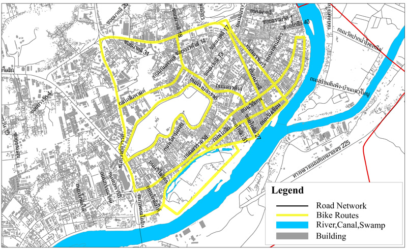
Nakhon Sawan Municipality is a district in Nakhon Sawan Province located in the central part of Thailand. It serves as a major transportation hub and gateway to the northern region. Its location is where the Ping and Nan Rivers converge and form the Chao Phraya River, the most important waterway of Thailand. Nakhon Sawan Municipality is one of the first cities in Thailand that place importance on promoting Non-Motorized Transport (NMT) in order to solve traffic congestion problems, reduce environmental impacts, and enhance sustainability. The people in Nakhon Sawan Municipality are seriously encouraged to ride bicycles for exercise and use bicycles as their daily transportation mode. Nakhon Sawan Municipality started building a bike route around Sawan Park for exercise purposes in 2013 [5, 7]. It also planned to expand the bike route network to cover the areas within a 20 kilometer radius of the city center [8] in order to make private car drivers change their daily transportation mode to bicycle. The bike route network was determined based on the results of a qualitative study that used the focus group discussion method to collect the opinions about the bike routes that are suitable for daily use [9]. The bike routes resulting from the qualitative research are shown in Fig. (1).
However, the results obtained from the focus group discussions solely reflected the needs of the key informants. An engineering data analysis has not been used to design appropriate bike lane patterns and evaluate the design of bike lane before actual construction. Thus, the present research intended to study the appropriateness of bike lanes in order to fulfill this knowledge gap and develop the guidelines for use in other cities of Thailand. The AIMSUN microscopic simulation software was used to simulate the traffic conditions of Nakhon Sawan Municipality. The forms of bike lane were categorized into 2 groups: 1) Conventional Bike Lane (CBL), which refers to a bike lane located on the left side of the main street and 2) Median Bike Lane (MBL), which refers to a bike lane located on the right side or center median of the street. The objective of this research was to analyze and compare the traffic conditions resulting from the AIMSUN microscopic simulation model, which could be divided into 3 cases: 1) existing road network with Non-Bike Lane (NBL), 2) road network with Conventional Bike Lane (CBL), and 3) road network with Median Bike Lane (MBL). The results would be used as efficiency data for analyzing the appropriate traffic demand of private cars and bicycles, evaluating project appropriateness, and determining campaign goals for a change in the mode of transportation from private car to bicycle.
This paper is organized as follows. Section 2 introduces the statement of problem. Section 3 presents the review of the literature. Section 4 describes how to carry out the field survey. Section 5 explains the process of creating the AIMSUN microscopic simulation model. Section 6 shows the comparative analysis of the traffic simulation data in all 3 cases. Section 7 gives a summary and conclusion of the present study.
2. STATEMENT OF PROBLEM
Due to the increasing traffic congestion problems and environmental impacts in the urban areas of Nakhon Sawan Municipality, there has been an attempt to sustainably solve this issue by encouraging private car drivers to change their daily transportation mode to bicycle. The bike route design ideas were mainly based on the quantitative research results concerning the daily transportation needs of the local people and the qualitative research results obtained from the focus group discussions with the key informants about appropriate bike routes for everyday use. However, the appropriateness and practical results of each bike lane form have not been systematically assessed before construction, leading to a lack of efficient and reasonable data to design bike routes and determine campaign goals and strategies that are in line with actual situations. This makes many cities in Thailand unsuccessful in creating campaigns to promote cycling and encouraging people to use the provided cycling infrastructure, which is considered a waste of budget and investment resources [10].
3. LITERATURE REVIEW
Research studies about the design of bike routes have been widely carried out. Most of them aim to study the physical suitability of bike lanes and the environment along cycling routes in order to promote the safety and convenience of cyclists and develop relevant facilities that suit the needs of cyclists aged 5-95 years [8]. D. Taylor and W. Davis [11] and many organizations reviewed basic research in bicycle traffic science in order to develop the design guidelines that are in line with engineering principles, for example, the width of bike lane should not be less than 1.2-1.5 meters [12], the speed limit within urban areas should not exceed 30 kilometers per hour [8], the conflict points on bike lanes should be painted with different color so that car drivers can clearly see them and drive more carefully [13-15], and the volume of motor vehicles in a bike lane should be less than 5,000 vehicles per day, when the posted travel speed does not exceed 60 kilometers per hour [16].
In addition, there are many quantitative and qualitative research studies that have been conducted with the following two main aims: 1) to study the factors affecting the behavior of cyclists and the shift of transportation mode to bicycle, which include safety, attractiveness of bike routes, surrounding environment of bike routes, easy accessibility to bike routes, and provision of parking spaces and related facilities [7, 9, 17-20], and 2) to examine the satisfaction and anxiety of cyclists after using a bike route, which is associated with road conditions, air conditions, air pollution, surrounding environment, accessibility, continuity of bike routes, linkage with other types of vehicles, parking spaces, traffic signs and equipment, barriers, lighting at night, maintenance spots, and risk of accidents and crimes [21-24].
However, there are only a few experimental and evaluative research studies on the design of bike routes that focus on creating traffic simulations with computer programs. Almost all of them pay attention to designing the physical features of an intersection in order to promote the safety of cyclists and minimize the transportation delay time. Robbin Blokpoel and Mahtab Joueiai used the SUMO - microscopic modeling of bicycle flow to design the infrastructure for safety of cyclists. Intersection topology is modified, when considering adding extra lanes to the bicycle path to allow cyclists to form lines and cross vehicle lanes with the traffic light [25]. David Stanek, PE and Charles Alexander, PE, and AICP evaluated the operations of relevant methods for controlling the interaction between right-turning vehicles and cyclists at a signalized protected intersection by using the Vissim microsimulation model [26]. In addition, Høsser placed importance on designing an intersection as the top priority of public transport, cyclists and pedestrians. Achieving increased efficiency through a new intersection design is considered as “throughabout”. Analyses of scenarios are performed in the AIMSUN traffic software [27]. Chalermwongphan and Upala created a traffic simulation model of Nakhon Sawan Municipality’s road network in order to find bicycle traffic demand estimation resulting from running dynamic O/D adjustment with the AIMSUN microscopic simulation software. The process of model calibration and validation was performed with the use of statistical measurement. The goodness-of-fit test was carried out to examine 9 measures. The data were analyzed using the multi-factor scoring method. The O/D matrix adjustment output of the scenario with the highest score was set as the estimated bicycle traffic demand between zones in Nakhon Sawan Municipality [10].
As the researchers recognized the knowledge gaps from the review of previous literature, the present research intended to compare and analyze appropriate forms of shared roadways by creating a model of Nakhon Sawan Municipality’s bike route network according to the qualitative results obtained from the focus group discussions [7, 9] with the use of the AIMSUN microscopic simulator. The results will be helpful in selecting an appropriate form of bike lane, assessing investment worthiness, and determining campaign goals for a change in the mode of transportation from private car to bicycle, which can ultimately contribute to solving traffic congestion problems and reducing environmental impacts in a sustainable way.
4. RESEARCH METHODOLOGY
4.1. Methodological Approach
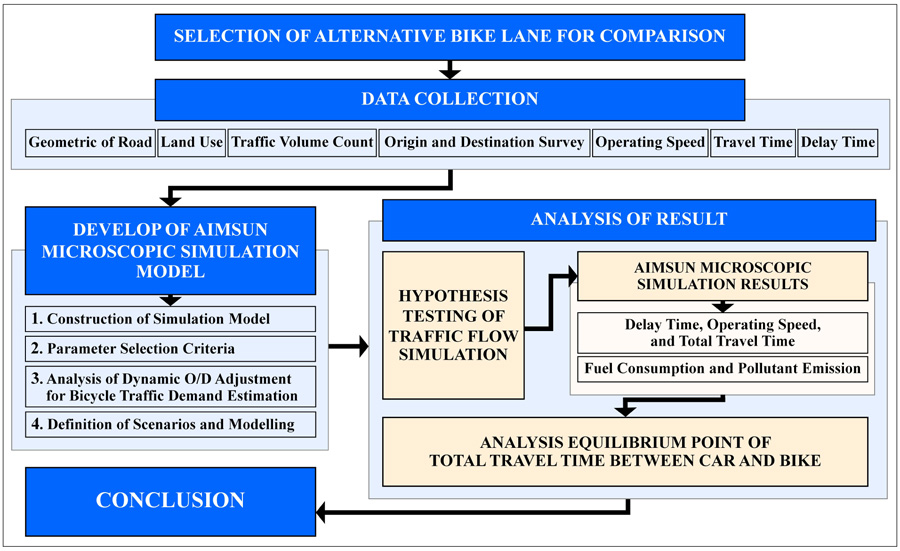
The present research was carried out according to the following 7 procedures: 1) selection of alternative bike lane for comparison, 2) field data collection, 3) development of AIMSUN microscopic simulation model, 4) hypothesis testing of traffic flow simulation, 5) obtaining AIMSUN microscopic simulation result, 6) analyzing equilibrium point of total travel time between car and bike, and 7) drawing conclusion. The detail is shown in Fig. (2)
4.2. Selection of Alternative Bike Lane for Comparison
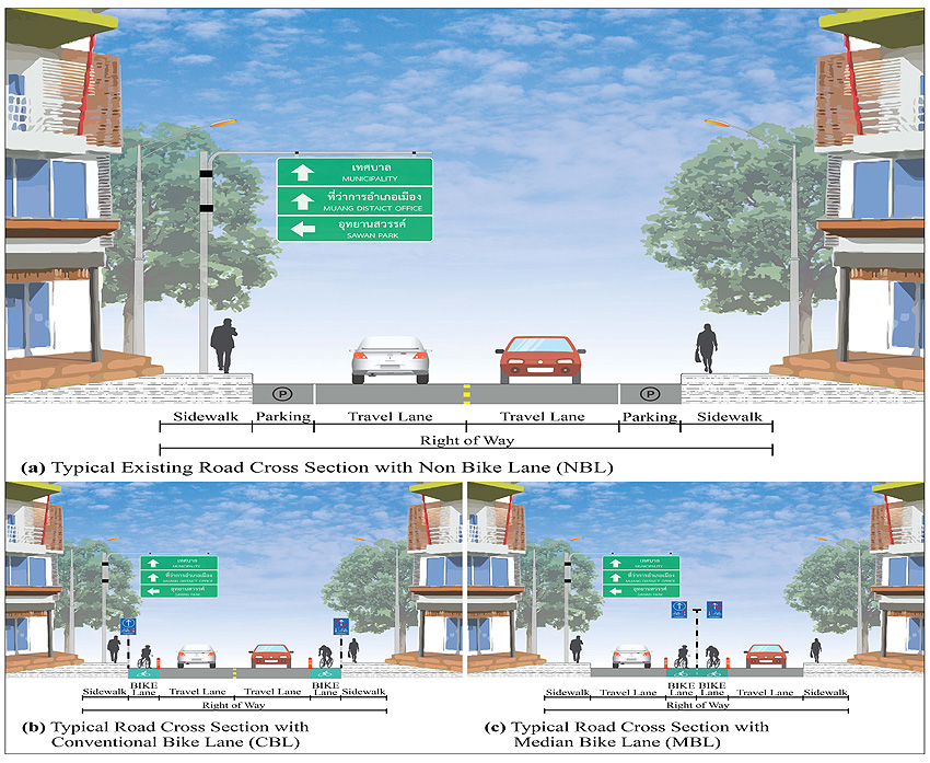
This research aimed to compare and evaluate two forms of shared roadways, which were 1) Conventional Bike Lane (CBL) located on the left side of the main road, and 2) Median Bike Lane (MBL) located on the right side or center median of the road. The on-street parking spaces were modified in order to support bike lanes. The size of the right of way was kept the same as before. The obstacles around the corners were removed. The physical conditions of intersections were adjusted to ensure that the turning angle was in line with the required standards. All bike routes were designed to connect together and comply with physical condition standards according to engineering principles. The results of the qualitative research concerning the appropriate bike routes for daily use [7, 9] were compared with the actual road network with non-bike lane. A traffic simulation model was created using the AIMSUN microscopic simulator. The simulated traffic conditions could be divided into 3 cases: 1) existing road network with Non-Bike Lane (NBL), 2) road network with a Conventional Bike Lane (CBL), and 3) road network with Median Bike Lane (MBL). The typical road cross-sections of these 3 cases are shown in Fig. (3).
4.3. Data Collection
Considering the survey of physical characteristics of roads in Nakhon Sawan Municipality, a functional classification system was applied to categorize the streets and highways in Nakhon Sawan Municipality into 4 groups according to the character of service they were intended to provide, which included 1) arterial streets, 2) collector streets, 3) local streets, and 4) transition ramps [28]. The morning peak period on weekends was chosen to be from 6:00 AM – 1:00 PM. The traffic data were surveyed based on the time period campaigned for reducing the use of private cars [7, 9]. The mid-block counts were conducted in 15-minute intervals at 54 locations and the vehicles were categorized into 8 groups. The observed traffic volume was subsequently converted into Passenger Car Unit (PCU) before importing to the database in form of Real Data Sets (ISO Format YYYY-MM-DDTHH: MM: SS) during the model calibration and validation process. The test vehicle techniques together with Car DVR Camera GPS were used to examine the travel speed and delay time [29, 30]. Moreover, the origin and destination survey was also carried out with the license plate matching techniques [31-33] in order to examine the traffic demand in Nakhon Sawan Municipality, which was classified into 17 zones based on land use purposes, for example, residential areas (i.e. houses, schools, hospitals, temple, etc.), commercial areas, recreation areas, and government officer areas [34].
4.4. Development of the AIMSUN Microscopic Simulation Model
AIMSUN Next Model is a program that has been widely used as a tool in experimental research. It can be applied to test research hypotheses by simulating a road network and defining transportation mode and management details. It has a process of virtual traffic simulation that is carried out based on internationally recognized theories and research results. Its virtual traffic simulation can be presented in both 2D and 3D views. Moreover, when each simulation scenario ends, all statistical and graphical results will be thoroughly displayed. AIMSUN Next Model is comprised of 3 main components: dynamic solution, microscopic simulator, mesoscopic and hybrid simulator that can deal with different traffic networks, including urban networks, freeways, highways, ring roads, arterials, and any combination thereof.
The microsimulator followed a microscopic simulation approach. Behavior of each vehicle in the network was continuously modeled throughout the simulation time period while it traveled through the traffic network, according to several vehicle behavior models such as car-following model, lane-changing model, gap acceptance model, and give way model. Environmental models, such as a fuel consumption model and the Panis et al emission model were also applied to evaluate fuel consumption and pollutant emission of each vehicle in every simulation step. The input data required by AIMSUN dynamic simulator was a simulation scenario. The simulation parameters were fixed values that described the experiment and some variable parameters used to calibrate the model [35]. The development of the AIMSUN microscopic simulation model had four key stages: (1) construction of simulation model, (2) parameter selection criteria, (3) model calibration and validation, and (4) definition of scenario and modeling.
4.4.1. Construction of Simulation Model
The road network map of Nakhon Sawan Municipality was created by importing Geographic Information System (GIS) data and a 1:4,000 scale aerial photograph [36] into the AIMSUN microscopic simulation software. Alignment of roads was modified to be in line with actual conditions. The functional classification of roads was applied to identify 712 links (roads) and 237 nodes (junctions). The attribute data of each road was determined based on the field survey data and the design standards such as design speed, capacity, lane width, and traffic management [12, 28, 37]. Nodes constituting intersections were set as yellow boxes in order to prevent queueing nodes from blocking other traffic [27]. Regarding the traffic control devices used in the unsignalized intersection, pavement markings and give way signs were used in minor roads to reduce speed when vehicles approached the intersection and let a driver on another approach proceed [38]. The developed road network map was used to simulate Case 1 (NBL) of traffic conditions.
In order to simulate Case 2 (CBL) and Case 3 (MBL), the physical characteristics of roads in Case 1 (NBL) were modified as follows. Roadside parking was replaced with a bike lane. The size of the right of way was controlled to be in line with the field survey data. The width of the bike lane was set to be between 1.50 - 2.00 meters according to the width of right way of each existing road [12]. The width of the bike lane mentioned above was able to serve the daily transportation needs of commuters at 30 km/h [8] without affecting other vehicles that traveled with a speed of less than 60 km/h on the major road [16].
4.4.2. Parameter Selection Criteria
The controllable parameters from previous research, which were consistent with this study, were used to indicate control criteria so as to make the model virtually identical with the studied areas. The details of parameter selection criteria are shown in Table 1.
4.4.3. Analysis of Dynamic O/D Adjustment for Bicycle Traffic Demand Estimation
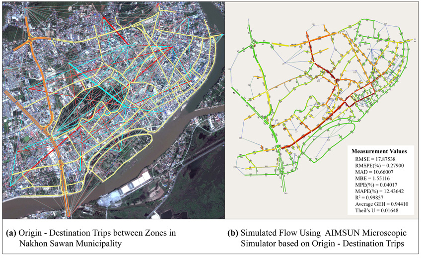
Regarding the traffic demand estimation, the O/D matrices of Case 1 (NBL) were adjusted through importing the origin and destination survey data into the AIMSUN microscopic simulation program, so as to stimulate 99 scenarios of dynamic O/D adjustment. The outcomes were thoroughly analyzed in order to select the best scenario for the model validation process. Quantitative validation can be performed with the use of statistical measurement, including the goodness-of-fit test. The 9 measures that were used to quantify the model predictive accuracy consisted of 1) Root Mean Square Error (RMSE), 2) Root Mean Square Percentage Error (RMSPE%), 3) Mean Absolute Deviation (MAD). 4) Mean Bias Error (MBE), 5) Mean Percentage Error (MPE%), 6) Mean Absolute Percentage Error (MAPE%), 7) Coefficient of Determination (R2), 8) GEH Statistic (GEH), and 9) Thiel’s U Statistic (Theil’s U). The results were analyzed using the multi-factor scoring method. The O/D matrix adjustment output of the scenario with the highest score was set as the estimated traffic demand between zones in Nakhon Sawan Municipality. The O/D matrix adjustment scenario with the highest score is shown in Fig. (4) [10].
4.4.4. Definition of Scenarios and Modelling
According to the analysis of dynamic O/D adjustment for bicycle traffic demand estimation in Case 1 (NBL), the traffic demand of private car commuters that traveled between 17 zones in Nakhon Sawan Municipality was at 15,384 cars per hour. In the present research, the researchers would call this value a 100% traffic demand. This data was used as the initial data for determining a hypothesis for analyzing and comparing the proportion of private cars and bicycles in Case 2 (CBL) and Case 3 (MBL). The data of cars (CAR) and bikes (BIKE) was required for running dynamic simulation experiments. The traffic demands of cars and bicycles would be examined and compared with a 100% traffic demand (15,384 cars per hour). The simulated traffic situations could be divided into 6 scenarios according to the percentage of CAR and BIKE as shown in Table 2.
| Main Parameters of Vehicle Attributes | ||||||||||||||||||||
| CAR | Mean | Deviation | Minimum | Maximum | References | |||||||||||||||
| Max Desired Speed | 89 km/h | 5 km/h | 85 km/h | 95 km/h | [35, 39, 40] | |||||||||||||||
| Max Acceleration | 2.70 m/s2 | 0.20 m/s2 | 2.20 m/s2 | 3.50 m/s2 | ||||||||||||||||
| Normal Deceleration | 3.5 m/s2 | 0.20 m/s2 | 3.00 m/s2 | 4.00 m/s2 | ||||||||||||||||
| Max. Deceleration | 6.00 m/s2 | 0.50 m/s2 | 5.00 m/s2 | 7.00 m/s2 | ||||||||||||||||
| BIKE | Mean | Deviation | Minimum | Maximum | References | |||||||||||||||
| Max Desired Speed | 25 km/h | 10 km/h | 20 km/h | 30 km/h | [8, 12, 35, 39, 41] | |||||||||||||||
| Max Acceleration | 1.50 m/s2 | 0.20 m/s2 | 1.00 m/s2 | 2.00 m/s2 | ||||||||||||||||
| Normal Deceleration | 2.20 m/s2 | 0.20 m/s2 | 1.40 m/s2 | 3.00 m/s2 | ||||||||||||||||
| Max. Deceleration | 3.00 m/s2 | 0.25 m/s2 | 2.00 m/s2 | 4.00 m/s2 | ||||||||||||||||
| Fuel Consumption Parameters of CAR | ||||||||||||||||||||
|
Fi (Idling) |
F1 (at 90 km/h) |
F2 (at 120 km/h) |
C1 (Accelerating) |
C2 (Accelerating) |
Fd (Decelerating) |
Minimum Consumption Speed: Vm |
References | |||||||||||||
| 0.330 (ml/s) |
4.700 (l/100 km) |
6.500 (l/100 km) |
0.420 (ml/s) |
0.260 (ml/s) |
0.537 (ml/s) |
50.000 (km/h) |
[35, 42-44] | |||||||||||||
|
Note: Fi is the fuel consumption rate for idling vehicles in ml/s. C1 and C2 are the two constants in the equation for the fuel consumption rate for accelerating vehicles, Fa, in ml/s. F1 is the fuel consumption rate, in liters per 10 km, for vehicles traveling at a constant speed of 90 km/h. F2 is the fuel consumption rate, in liters per 10 km, for vehicles traveling at a constant speed of 120 km/h. Vm is the speed at which the fuel consumption rate, in ml/s, is at a minimum for vehicles for a vehicle cruising at a constant speed. Fd is the fuel consumption rate for decelerating vehicles in ml/s. |
||||||||||||||||||||
| Pollution Emission Parameters of CAR | ||||||||||||||||||||
| Pollutant | Fuel Type | Acceleration | Lower Limit | Factor 1 | Factor 2 | Factor 3 | Factor 4 | Factor 5 | Factor 6 | References | ||||||||||
| CO2 | Petrol | - | 0 | 5.53e-01 | 1.61e-01 | -2.89e-03 | 2.66e-01 | 5.11e-01 | 1.83e-01 | [35, 45, 46] | ||||||||||
| NOx | Petrol | a ≥ -0.5 m/s2 | 0 | 6.19e-01 | 8.00e-05 | -4.03e-06 | -4.13e-04 | 3.80e-04 | 1.77e-04 | |||||||||||
| Petrol | a < -0.5 m/s2 | 0 | 2.17e-04 | 0.00e+00 | 0.00e+00 | 0.00e+00 | 0.00e+00 | 0.00e+00 | ||||||||||||
| VOC | Petrol | a ≥ -0.5 m/s2 | 0 | 4.47e-03 | 7.32e-07 | -2.87e-08 | -3.41e-06 | 4.94e-06 | 1.66e-06 | |||||||||||
| Petrol | a < -0.5 m/s2 | 0 | 2.63e-03 | 0.00e+00 | 0.00e+00 | 0.00e+00 | 0.00e+00 | 0.00e+00 | ||||||||||||
| PM | Petrol | - | 0 | 0.00e+00 | 1.57e-05 | -9.21e-07 | 0.00e+00 | 3.75e-05 | 1.89e-05 | |||||||||||
| Vehicle Type | Percentage of Traffic Demand Assignment | |||||
|---|---|---|---|---|---|---|
| Scenario 1 | Scenario 2 | Scenario 3 | Scenario 4 | Scenario 5 | Scenario 6 | |
|
CAR (car/hr) (Percentage of CAR) |
15,384 (100%) |
13,867 (90%) |
12,3280 (80%) |
10,824 (70%) |
9,294 (60%) |
7,787 (50%) |
|
BIKE (bike/hr) (Percentage of BIKE) |
- (0%) |
1,682 (10%) |
3,182 (20%) |
4,696 (30%) |
6,203 (40%) |
7,787 (50%) |
Considering the running of micro stochastic route choice experiments, the path assignment was set to be constant values resulting from running dynamic user equilibrium, which would be used to control the behavioral factors affecting route selection and the time intervals between two consecutive vehicle arrivals (headway) at input sections that were sampled from a truncated normal distribution [10]. Ten replications of each scenario were performed to find the average value. When comparing the the same scenario results of Case 2 (CBL) and Case 3 (MBL) with the student’s t-test method [47-49] in Stata Software [50], the traffic flow simulation of CAR and BIKE must be equal at a statistical significance level of 5% (α = 5%). This was to control the independent variables and avoid errors that might arise from gridlock phenomena in the center of an intersection during a traffic simulation [51]. To test the equality under the null hypothesis with a confidence level of 95%, the result of Traffic FlowCBL and Traffic FlowMBL measurements, H0: Traffic FlowCBL = Traffic FlowMBL against H1: Traffic FlowCBL ≠ Traffic FlowMBL at a statistical significance level of 5% (α = 5%).
|
Traffic Scenario |
Traffic Flow Simulation | ||||
|---|---|---|---|---|---|
| (NBL) | (CBL) | (MBL) | |||
| CAR (car/hr) | CAR (car/hr) | BIKE (bike/hr) | CAR (car/hr) | BIKE (bike/hr) | |
| Scenario 1 | 15137.57 | 15137.60 | - | 15137.60 | - |
| Scenario 2 | 15137.57 | 13638.60 | 1632.70 | 13638.60 | 1638.70 |
| Scenario 3 | 15137.57 | 12137.50 | 3111.10 | 12137.46 | 3109.00 |
| Scenario 4 | 15137.57 | 10641.08 | 4605.62 | 10641.06 | 4595.75 |
| Scenario 5 | 15137.57 | 9138.21 | 6095.36 | 9138.17 | 6088.42 |
| Scenario 6 | 15137.57 | 7648.73 | 7592.45 | 7648.80 | 7580.80 |
CBL is Case 2 of simulated traffic conditions (road network with Conventional Bike Lane).
MBL is Case 3 of simulated traffic conditions (road network with Median Bike Lane).
|
Comparison of Traffic Flow Simulation |
Paired t-test (Difference Value) | t | df | Pr(|T| > |t|) | ||||
|---|---|---|---|---|---|---|---|---|
| Mean | Std. Err. | Std. Dev. | 95% Conf. Interval | |||||
| CAR(CBL) - CAR(MBL) | 0.005 | 0.017 | 0.409 | -0.377 | 0.048 | 0.307 | 5 | 0.771 |
| BIKE(CBL) - BIKE(MBL) | 4.912 | 3.171 | 7.090 | -3.891 | 13.716 | 1.549 | 4 | 0.196 |
5. ANALYSIS OF THE RESULTS
5.1. Hypothesis Testing of Traffic Flow Simulation
After testing Case 2 (CBL) and Case 3 (MBL) with various traffic demands of CAR and BIKE in 6 scenarios according to the hypothesis, the traffic flow simulation results can be summarized in Table 3.
The traffic flow simulation values of CAR and BIKE in each scenario were compared and analyzed using the student’s t-test in Stata Program in order to confirm the accuracy of the results and ensure that the results were consistent with the hypothesis. The details are shown in Table 4.
Based on the student’s t-test results, it was found that the null hypothesis is accepted, considering that the average traffic flow simulation values of CAR and BIKE in Case 2 (Traffic FlowCBL) were equal to those in Case 3 (Traffic FlowMBL) at a statistical significance level of 5% (Car = Mean Difference 0.005%; 95%CI -0.377 to 0.048, P-value = 0.771 and Bike = Mean Difference 4.912%; 95%CI -3.891 to 13.716, P-value = 0.196). This was in line with the hypothesis that was set to control the independent variables and avoid errors from gridlock phenomena during the simulation of traffic conditions.
5.2. AIMSUN Microscopic Simulation Results
5.2.1. Delay Time, Operating Speed, and Total Travel Time
Table 5 shows the simulation of traffic conditions in AIMSUN microscopic simulation model and the comparative analysis results of the difference (Diff.*(CBL)) between Case 1 (NBL) and Case 2 (CBL) as well as the difference (Diff.*(MBL)) between Case 1 (NBL) and Case 3 (MBL) in the aspects of delay time, operating speed, and total travel time. It was found that, in Scenario 1 with a 100% CAR traffic demand (1,538 veh/h), the delay time of CAR in Case 2 (CBL)CAR and Case 3 (MBL)CAR was 9.85 sec/km and 10.84 sec/km, respectively. The delay time of CAR in Case 2 and Case 3 was found to decrease, when compared with Case 1, considering that Diff.*(CBL)CAR = 1.33 sec/km and Diff.*(MBL)CAR = 0.34 sec/km. The delay time of CAR in Case 2 and Case 3 dramatically reached a trough in Scenario 2 when reducing the percentage of CAR traffic demand to 90% (13,867 veh/h) and importing the BIKE traffic demand of 10% (1,682 veh/h), considering that (CBL)CAR = 9.28 sec/km, (Diff.*(CBL)CAR = 1.90 sec/km, (MBL)CAR = 9.92 sec/km, and (Diff.*(MBL)CAR = 1.26 sec/km. After that, the delay time of CAR was continually increasing, when the percentage of CAR traffic demand was reduced and the percentage of BIKE traffic demand increased on a continuous basis. In Scenario 6, when the percentages of CAR traffic demand and BIKE traffic demand were equivalent at 50% (7,787 veh/h), the delay time of CAR in Case 2 (CBL)CAR was 0.91 sec/km (Diff.*(CBL)CAR = 0.71 sec/km) and the delay time of CAR in Case 3 (MBL)CAR was 10.98 sec/km (Diff.*(CBL)CAR = 0.20 sec/km).
As for the delay time of BIKE in Case 2 and Case 3, when importing the BIKE traffic demand of 10% (1,682 veh/h) in Scenario 2, the delay times of both cases were similar at 14.20 sec/km and showed a tendency to constantly increase, related to the import of BIKE traffic demand in each scenario.
However, when comparing Case 2 (CBL) and Case 3 (MBL) in 6 scenarios, the results clearly showed that the average delay time of Case 2 (locating a bike lane on the left side of the main road) was lower than that of Case 3 (locating a bike lane on the center median of the road) by 0.70 sec/km with a highly significance level of less than 0.001 (P-Value < 0.001) [52, 53]. The delay time was due to the operating speed at a highly significant level (Pearson’s Correlation Coefficient > 0.90) in the opposite direction [54]. The average CAR operating speed of Case 2 (CBL)CAR was higher than that of Case 3 (MBL)CAR by 0.35 km/h with a highly significant level of P-value < 0.001. The average BIKE delay time of Case 2 was not different from that of Case 3 at a significance level of 5% (α = 5%). On the other hand, the average BIKE operating speed of Case 2 (CBL)BIKE was higher than that of Case 3 (MBL)BIKE by 0.10 km/h with a significance level of less than 0.05 (P-Value < 0.05).
|
Traffic Scenario |
Delay Time | Operating Speed | Total Travel Time | ||||||||||||
|---|---|---|---|---|---|---|---|---|---|---|---|---|---|---|---|
|
Car (sec/km) |
Bike (sec/km) |
Car (km/h) |
Bike (km/h) |
Car (h) |
Bike (h) |
||||||||||
| (NBL) | (CBL) | (MBL) | (CBL) | (MBL) | (NBL) | (CBL) | (MBL) | (CBL) | (MBL) | (NBL) | (CBL) | (MBL) | (CBL) | (MBL) | |
| Scenario 1 | 11.18 | 9.85 | 10.84 | - | - | 48.10 | 48.85 | 48.43 | - | - | 599.42 | 593.66 | 594.32 | - | - |
| Diff.* | 1.33 | 0.34 | -0.75 | -0.33 | 5.76 | 5.10 | |||||||||
| Scenario 2 | 11.18 | 9.28 | 9.92 | 14.20 | 14.22 | 48.10 | 49.07 | 48.73 | 26.35 | 26.28 | 599.42 | 531.54 | 530.09 | 12.42 | 124.89 |
| Diff.* | 1.90 | 1.26 | -0.97 | -0.63 | 67.88 | 69.33 | |||||||||
| Scenario 3 | 11.18 | 9.54 | 10.21 | 24.19 | 24.11 | 48.10 | 48.89 | 48.55 | 24.52 | 24.47 | 599.42 | 474.95 | 474.46 | 254.74 | 254.68 |
| Diff.* | 1.64 | 0.97 | -0.79 | -0.45 | 124.47 | 124.96 | |||||||||
| Scenario 4 | 11.18 | 9.84 | 10.48 | 32.14 | 31.76 | 48.10 | 48.73 | 48.39 | 23.33 | 23.26 | 599.42 | 419.27 | 418.40 | 398.12 | 395.33 |
| Diff.* | 1.34 | 0.70 | -0.63 | -0.29 | 180.15 | 181.02 | |||||||||
| Scenario 5 | 11.18 | 10.07 | 10.66 | 38.5 | 39.05 | 48.10 | 48.62 | 48.3 | 22.38 | 22.29 | 599.42 | 360.61 | 360.42 | 545.92 | 547.23 |
| Diff.* | 1.11 | 0.52 | -0.52 | -0.20 | 238.81 | 239.00 | |||||||||
| Scenario 6 | 11.18 | 10.27 | 10.98 | 44.26 | 45.32 | 48.10 | 48.48 | 48.15 | 21.63 | 21.41 | 599.42 | 303.81 | 303.84 | 703.04 | 709.99 |
| Diff.* | 0.91 | 0.20 | -0.38 | -0.05 | 295.61 | 295.58 | |||||||||
▪ Non-Bike Lanes (NBL) CAR and Conventional Bike Lanes (CBL) CAR calculated as: Diff.*(CBL)CAR = (NBL)CAR – (CBL)CAR.
▪ Non-Bike Lanes (NBL) CAR and Median Bike Lanes (MBL) CAR calculated as: Diff.*(MBL)CAR = (NBL)CAR – (MBL)CAR.
|
Traffic Scenario |
Fuel Consumption and Pollutant Emission Rate | ||||||||||||||
|
Fuel Consumption (l) |
CO2 (g/km) |
NOX (g/km) |
PM (g/km) |
VOC (g/km) |
|||||||||||
| (NBL) | (CBL) | (MBL) | (NBL) | (CBL) | (MBL) | (NBL) | (CBL) | (MBL) | (NBL) | (CBL) | (MBL) | (NBL) | (CBL) | (MBL) | |
| Scenario 1 | 3,195.66 | 3,058.63 | 3,025.40 | 7,466,825.84 | 7,335,318.35 | 7,219,963.02 | 23,355.96 | 22,924.91 | 22,617.88 | 3,744.00 | 3,565.90 | 3,505.60 | 3,854.78 | 3,833.94 | 3,823.66 |
| %Diff.* | 4.29% | 5.33% | 1.76% | 3.31% | 1.85% | 3.16% | 4.76% | 6.37% | 0.54% | 0.81% | |||||
| Scenario 2 | 3,195.66 | 2,723.97 | 2,730.54 | 7,466,825.84 | 6,552,181.03 | 6,503,285.82 | 23,355.96 | 20,578.94 | 20,309.76 | 3,744.00 | 3,150.05 | 3,138.24 | 3,854.78 | 3,425.66 | 3,439.11 |
| %Diff.* | 14.76% | 14.55% | 12.25% | 12.90% | 11.89% | 13.04% | 15.86% | 16.18% | 11.13% | 10.78% | |||||
| Scenario 3 | 3,195.66 | 2,429.60 | 2,450.71 | 7,466,825.84 | 5,840,660.79 | 5,827,160.92 | 23,355.96 | 18,293.23 | 18,231.72 | 3,744.00 | 2,802.15 | 2,844.52 | 3,854.78 | 3,077.81 | 3,059.35 |
| %Diff.* | 23.97% | 23.31% | 21.78% | 21.96% | 21.68% | 21.94% | 25.16% | 24.02% | 20.16% | 20.63% | |||||
| Scenario 4 | 3,195.66 | 2,143.41 | 2,166.64 | 7,466,825.84 | 5,146,902.28 | 5,145,879.81 | 23,355.96 | 16,168.16 | 16,073.42 | 3,744.00 | 2,475.89 | 2,520.34 | 3,854.78 | 2,705.87 | 2,699.65 |
| %Diff.* | 32.93% | 32.20% | 31.07% | 31.08% | 30.78% | 31.18% | 33.87% | 32.68% | 29.80% | 29.97% | |||||
| Scenario 5 | 3,195.66 | 1,844.39 | 1,872.00 | 7,466,825.84 | 4,426,682.50 | 4,444,426.41 | 23,355.96 | 13,866.09 | 13,883.61 | 3,744.00 | 2,127.10 | 2,181.14 | 3,854.78 | 2,341.81 | 2,329.94 |
| %Diff.* | 42.28% | 41.42% | 40.72% | 40.48% | 40.63% | 40.56% | 43.19% | 41.74% | 39.25% | 39.56% | |||||
| Scenario 6 | 3,195.66 | 1,551.51 | 1,587.40 | 7,466,825.84 | 3,722,692.32 | 3,756,228.49 | 23,355.96 | 11,654.81 | 11,695.26 | 3,744.00 | 1,786.65 | 1,847.67 | 3,854.78 | 1,975.98 | 1,967.61 |
| %Diff.* | 51.45% | 50.33% | 50.14% | 49.69% | 50.10% | 49.93% | 52.28% | 50.65% | 48.74% | 48.96% | |||||
§ Non-Bike Lanes (NBL) CAR and Conventional Bike Lanes (CBL) CAR calculated as:
Diff.*(CBL)CAR =
§ Non-Bike Lanes (NBL) CAR and Median Bike Lanes (MBL) CAR calculated as:
Diff.*(MBL)CAR =
In addition, the results suggested that a change in transportation mode from private car to bicycle could make the average total travel time increase at a statistical significance level (P-Value ≈ 0.02), depending on the increase in the percentage of BIKE in each scenario. Meanwhile, the location of the bike lane in Case 2 (CBL) and Case 3 (MBL) did not have an effect on the average total travel time of CAR and BIKE at a statistical significance level of 5% (α = 5%).
5.2.2. Fuel Consumption and Pollutant Emission
The simulation of 3 traffic cases also revealed the data about fuel consumption (liter) and emission of pollutants (g/km), including carbon dioxide (CO2), nitrogen oxides (NOX), Particulate Matter (PM), and Volatile Organic Compounds (VOC). According to the analysis results of the percentage difference (%Diff.*(CBL)) between Case 1 (NBL) and Case 2 (CBL) as well as the percentage difference (%Diff.*(MBL)) between Case 1 (NBL) and Case 3 (MBL) shown in Table 6, it was found that the average fuel consumption and pollutant emission rate of CAR in Case 2 was not different from that of CAR in Case 3 at a significance level of 5% (α = 5%).
Therefore, in order to present the research results in a clearer way, the average difference values of Case 2 (CBL) and Case 3 (MBL) were calculated and compared with the values of Case 1 (NBL). In Scenario 1, where the full traffic demand was at 1,538 veh/h, the average difference values of Case 2 (CBL) and Case 3 (MBL) in the aspects of fuel consumption and emission of carbon dioxide (CO2), nitrogen oxides (NOX), particulate matter (PM), and volatile organic compounds (VOC) were lower than those of Case 1 (NBL) at 153.65 liter (4.81%), 189,185.16 g/km (2.53%), 584.57 g/km (2.50%), 208.25 g/km (5.56%), and 25.98 g/km (0.67%), respectively and tended to continuously decrease according to the decrease in proportion of CAR in each scenario.
5.2.3. Analyzing Equilibrium Point of Total Travel Time between CAR and BIKE
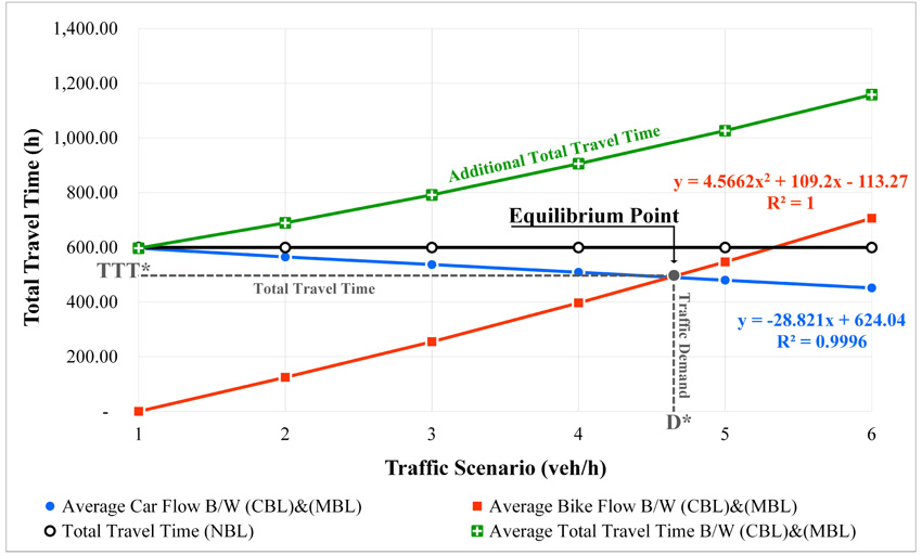
Regarding the analysis of appropriate CAR and BIKE traffic demands that should be used to determine campaign goals for a change in mode of transportation from private car to bicycle, the researchers took in to account the equilibrium point or the point of intersection between the traffic demand (traffic scenario) and the total travel time of CAR and BIKE in the graph, when CAR and BIKE spent the same amount of time in the road network. The average values of Case 2 (CBL) and Case 3 (MBL) obtained from the calculation were used to plot a graph of relationships as shown in Fig. (5).
Considering the equilibrium point between the total travel times of CAR and BIKE, it was found that the total travel time lines intersect at 490.54 h. The traffic demand values (D*) of CAR and BIKE were calculated to be 9,691 veh/hr and 5,543 veh/hr, which accounted for 36% of private cars that should change their transportation mode to bicycle. This could reduce the total travel time of CAR during peak hours by 108.88 h. and increase the total travel time of BIKE by 490.54 h. The overall total travel time was found to be higher than that of Case 1 (NBL) by 381.66 h. as reflected in the Average Total Travel Time B/W (CBL)&(MBL) or “Additional Total Travel Time” line within in Fig. (5).
CONCLUSION
Conducting campaigns for a change in daily transportation mode from private car to bicycle is another approach to sustainably solve traffic congestion problems and reduce environmental impacts. The present research aimed to analyze the outcomes resulting from using two different forms of bike lanes, conventional bike lane (Case 2; CBL) and median bike lane (Case 3; MBL), and then compare them with the existing road network with no bike lane (Case 1; NBL). The AIMSUN microscopic simulator was used to create the virtual traffic simulation model. The following conclusions were drawn based on the findings of this study.
- Regarding the physical characteristics of roads after modification, it was found that adding the conventional bike lane (Case 2; CBL) and median bike lane (Case 3; MBL) made the size of the turning circle at the intersection wider, resulting in more driving agility. When comparing the traffic simulation results of Case 1 (NBL) with Case 2 (CBL) and Case 1 (NBL) with Case 3 (MBL), it was found that the delay time, operating speed, total travel time, fuel consumption, and emission of carbon dioxide (CO2), nitrogen oxides (NOX), Particulate Matter (PM), and Volatile Organic Compounds (VOC) of CAR started to decrease during Scenario 1 with a 100% traffic demand of CAR and subsequently continued to decrease depending on the decrease in traffic demand of CAR in each scenario.
- Locating a bike lane on the left side of the main road (Case 2; CBL) made the average delay time of CAR lower than locating a bike lane on the center median of the main road (Case 3; MBL) by 0.70 sec/km. However, there was no difference in the average delay times of CAR in Case 2 and Case 3.
- The average operating speed of CAR and BIKE in Case 2 was higher than that of CAR and BIKE in Case 3 (CAR = 0.35 km/h and BIKE = 0.10 km/h).
- The decrease in the percentage of CAR and the increase in the percentage of BIKE in each scenario made the average total travel time of the entire road network higher.
- The average fuel consumption and emission of carbon dioxide (CO2), nitrogen oxides (NOX), particulate matter (PM), and volatile organic compounds (VOC), resulting from comparing the outcomes of Case 2 and Case 3 with Case 1, were found to continually increase according to the decrease in percentage of CAR in each scenario.
- The equilibrium point between the total travel times (TTT*) of CAR and BIKE was observed to be 490.54 h. The traffic demand values (D*) of CAR and BIKE were calculated to be 9,691 veh/hr and 5,543 veh/hr. As a result, the total travel time of CAR during peak hours could be reduced by 108.88 h., whereas the total travel time of BIKE was found to increase by 490.54 h. The overall total travel time was higher than that of Case 1 by 381.66 h. as reflected in the Average Total Travel Time B/W (CBL)&(MBL) or “Additional Total Travel Time” line within in Fig. (5).
The comparative analysis of 8 variables in Case 2 (CBL) and Case 3 (MBL) was conducted to select the best form of bike lanes. The results are summarized in Table 7.
| NO. | Variable | Vehicle Type | |||
|---|---|---|---|---|---|
| CAR | BIKE | ||||
| (CBL) | (MBL) | (CBL) | (MBL) | ||
| 1 | Delay Time (sec/km) |
 |
- | Equivalent | |
| 2 | Operating Speed (km/h) |
|
- |
 |
- |
| 3 | Total Travel Time (h) | Equivalent | Equivalent | ||
| 4 | Fuel Consumption (l) | Equivalent | - | - | |
| 5 | Carbon Dioxide (CO2) (g/km) | Equivalent | - | - | |
| 6 | Nitrogen Oxides (NOX) (g/km) | Equivalent | - | - | |
| 7 | Particulate Matter (PM) (g/km) | Equivalent | - | - | |
| 8 | Volatile Organic Compounds (VOC) (g/km) | Equivalent | - | - | |
The best value of CAR resulting from comparing (CBL)CAR with (MBL)CAR. The best value of BIKE resulting from comparing (CBL)BIKE with (MBL)BIKE.Equivalent: No statistically significant difference between Case 2 (CBL) and Case 3 (MBL).
Based on the research results, the Conventional Bike Lane (CBL) had the average delay time and operating speed that were more suitable for use than the Median Bike Lane (MBL). A campaign for a change in daily transportation mode from private car to bicycle should focus on reducing at least 9,691 veh/hr or 36% of all private cars in the road network. This approach could reduce the delay time by 0.89 sec/km, minimize the fuel consumption by 1,228.66 liters, and decrease the emission of carbon dioxide (CO2), nitrogen oxides (NOX), particulate matter (PM), and volatile organic compounds (VOC) by 2,769,764.47 g/km, 8654.86 g/km, 1,463.33 g/km, and 1,383.93 g/km respectively.
However, in order to convert on-street parking into bike lanes without affecting land use on both sides of the road and reduce social conflicts that may occur, the Thai government should prepare enough parking spaces within a radius of 500 meters from major spots with a lot of activities such as residential areas and business and service zones and also establish a reliable security system. This is to ensure that a campaign to promote cycling and encourage people to use the provided cycling infrastructure can be successfully carried out in a practical way.
As this research only focused on an overall road network system, future research should be conducted to specifically analyze the safety and delay times of Conventional Bike Lane (CBL) and Median Bike Lane (MBL) at intersections through creating a traffic simulation model with computer programs. This will be helpful in designing an efficient intersection that can promote safety and reduce transportation delays and beneficial for motivating people to use bicycles in their daily life in the future.
DISCLOSURE
Any opinions, findings, summary and conclusions expressed in this paper are those of the authors.
CONSENT OF PUBLICATION
Not applicable.
AVALIBILTY OF DATA AND MATERIAL
The data used to support the findings of this study are included in the article.
FUNDING
None.
CONFLICT OF INTEREST
The authors declare no conflict of interest, financial or otherwise.
ACKNOWLEDGEMENTS
Declared none.

