All published articles of this journal are available on ScienceDirect.

Congestion and Pollution, Vehicle Routing Problem of a Logistics Provider in Thailand
Abstract
Aim and Objective:
This study aims to minimise the travelling distance, operation cost in terms of fuel consumption, and CO2 emissions. It introduces the Time-Dependency Pollution-Routing Problem (TDPRP) with the implementation of the time-dependency and emission model, including constraints such as the limitation of vehicle capacity and vehicle’s speed during different time periods in Thailand. Furthermore, the time window constraint is applied for representing a more realistic model. The main objective is to minimise the total pollution generated because of transportation.
Methods:
The Genetic Algorithm (GA) and Tabu Search (TS) methods have been used to generate the optimal solution with a variety of experiments. The best solutions from all the experiments have been compared to the original solution in terms of the quality of the solution and the computation time.
Results:
The best solution was generated by using the TS method with 30,000 trials. The minimum of the total CO2 emissions was 183.9846 kilograms produced from all of the vehicles during transportation, nearly half from the current transportation plan, which produced 320.94 kilograms of CO2 emissions.
Conclusion:
The proposed model optimised both the route and schedules (multiple time periods) for a number of vehicles, for which the transportation during a fixed congestion period could be predicted to avoid traffic congestion and reduce the CO2 emission. Future research is suggested to add other specific algorithms as well as constraints in order to make the model more realistic.
1. INTRODUCTION
Nowadays, the greenhouse gas effect is one of the biggest world problems that every organisation needs to be concerned with. Green practices, besides, are interesting issues to study [1]. There are a lot of gases that are induced by Greenhouse Gas (GHG) emissions. However, human health and the depletion of the ozone layer are mostly affected by carbon dioxide (CO2) emissions. Cargo transportation is another way to create a lot of pollution. Especially, from road freight with emissions at about 78% of the emissions from all transport modes [2]. CO2 emissions are the result of fuel consumption and vehicle speed (travelling time). Transportation is the fastest-growing major contributor to global climate change, accounting for 23% of energy-related carbon dioxide (CO2) emissions. Many experts foresee a three- to five-fold increase in CO2 emissions from transportation in Asian countries by 2030 compared with emissions in 2000 if no changes are made to investment strategies and policies [3]. Traffic congestion directly affects the vehicle speed and the total time spent on the road. In addition, the fuel consumption rate depends on two factors, which are the speed of the vehicle and the load of the vehicle [4].
Many capital cities around the world have a problem with traffic congestion. Thailand’s capital city, Bangkok, is the worst city for traffic congestion. Especially, during the peak morning hours when traffic exhaust is blamed for the haze. It causes Bangkok to experience some of the worst-ever air pollution levels, caused by ultra-fine dust particles known as PM2.5 [5]. As a result, transporting goods in Bangkok is very difficult. This is due to the period of time specified by the customer to receive their products and also the quality of the products on the vehicle decreasing over time. Therefore, logistics companies need a good transportation plan in order to give better service and maintain the product’s quality. In addition, CO2 can be reduced by having a transportation plan. Governments and businesses are increasingly interested in the environment. Society recognises the environmental damage caused by human activities in businesses. Environmental Transport is one of the most visible aspects of the supply chain [6]. The amount of CO2 emitted from transportation, approximately 14% of emissions, is also the main source of nitrogen dioxide (NOx), sulphur dioxide (SO2), and other particles [7]. The results of the study of the most important factors for CO2 emissions in road transport were presented in [8].
Due to traffic congestion directly affecting the change in vehicle speed during peak times in big cities, the piecewise function has been used to capture the rules of different speeds of vehicles, which are very important in creating fuel consumption models and CO2 emissions. Therefore, efficient logistics and supply chain management could be the best transportation management for consumables and finished products. Transportation costs have a direct impact on prices. If firms can minimise such costs, they can acquire competitive products and also become an environmentally friendly company. Therefore, the interest in pollution routes with congestion problems has a significant increase in business operations. Companies are benefiting from the implementation of the Pollution Route Problem (PRP) model by reducing costs as well as developing product quality, reducing risks, and improving financial performance [9, 10].
Another aspect that has received attention is the integration of technological innovations in Vehicle Routing Problem (VRP) solutions. These include global location systems using computer data processing with high capacity and various techniques, which can be used to solve the model problem, such as the local search-based meta-heuristic technique, Genetic Algorithm (GA), and Tabu Search (TS) [11, 12]. The Vehicle Routing Problem is basically about mathematical models to solve the problem to achieve an optimal solution which is the minimum total cost. The Vehicle Routing Problem model became widely known and used after it was presented by [13]. Many other versions of the invention relate to real-world problems, such as the ability of a vehicle during a limited time in which each customer must be served, and traffic congestion. The recent model is about pollution and is called the Pollution Routing Problem (PRP). However, not many studies have been conducted in this area. Therefore, it is a challenge to work on this topic because not much information related to this topic can be found and the implementation of an accurate emission model is difficult. There are a few emission models which are available in the literature but all of them are very difficult to understand. Moreover, a lot of specific parameters are required in order to come to an accurate calculation. Another important factor is traffic congestion as it directly affects vehicle speed. In addition, the consumption rate (or CO2 emission rate) depends on two factors which are vehicle speed and vehicle load [4]. However, transportation during a fixed congestion period can be predicted.
This study introduces the Time-Dependency Pollution-Routing Problem (TDPRP), which implements the time-dependency and emission model in which it suits the characteristics of the case in Thailand. This model aims to minimise the total pollution that is generated by transportation. The time-dependency and emission models have been integrated in this work. The work may be similar to other research, but this study has focused more on the three hard constraints of the maximum load capacity, delivering products within a specific time window, and time-dependence, which are implemented in this model. The experimental case used the information provided by the logistics provider company in Thailand. They distribute perishable-products to customers around Bangkok. The main aim of this research was the implementation of an optimisation model for the pollution VRP with congestion, and it has proposed Genetic algorithms and Tabu search methods. The computation time and the results generated by the two methods needed to be compared. The results can be used in the future as an important decision factor in logistics planning and management, and business relief in both pollution and cost reduction.
This paper considered a general case of the transporting of goods, which were perishable goods, from a distributor that produced stock and delivered it to all the retailers around Bangkok, Thailand. Besides that, the traffic problem in Bangkok was one of the most important factors that needed to be considered, especially in the rush hour which can be divided into two periods, 5:30 am - 10 am and 4 pm - 8 pm. Since the products were perishable goods, hence, the quality of the products was very important. In order to achieve that constraint, there needed to be a good transportation plan to deliver the goods before or exactly on time. Since the goal of every company is to reduce operating costs to increase profits, decreasing travel distance for each truck would enable the company to lessen its operating costs in terms of fuel consumption. The travelling distance starts from the depot with a full truckload and delivers goods to the retailers that are assigned in the route. Moreover, the aim of the study was to minimise the pollution that was generated over the route. In some countries, logistics companies need to pay an emission tax to the government, therefore, this can help to reduce the operation cost. However, there is no policy about paying the emission cost in Thailand at present. Moreover, there are limited vehicles for product distribution. Their main customers are convenience store chains and fresh marts around Bangkok, which sell frozen food. Every day, the company will receive orders from the customers from the head office. The company will then have to assign the orders to the vehicles. All routes should start and end at the warehouse while each customer will receive one-time delivery service. In addition, customers will be arranged within a specified time-window, a time when customers are ready to receive the product. The objective function of a plan is, therefore, to minimise the total emission, and all the constraints must not be exceeded.
The remaining sections of this paper are structured as follows. Section 2 provides a review of the literature and previous studies of the VRP, VRPTW, TDVRP, PRP, and technical methodologies. Section 3 then describes the problem description and modelling. Section 4 suggests the study area and dataset used in this work. Finally, section 5 presents the results of the computational study for a set of proposed scenarios.
2. LITERATURE REVIEW
2.1. Vehicle Routing Problem (VRP)
The vehicle routing problem (VRP) was first launched by [13]. The VRP is one of the most important and challenging tasks to increase performance in a clear industry. It is in the category of NP-hard problems. The basic goal of the VRP algorithm is optimisation objectives, such as reducing the number of vehicles or the total length of the routes that can measure the distance (i.e., miles) and travel time (i.e., hours). A number of specific conditions must be considered, such as the capacity of each vehicle and that each customer has the exact requirements that must be satisfied. In addition, a classic VRP can be changed by adding constraints such as limited vehicle capacity, the length of time that each customer must receive service, and traffic congestion. Such constraints are the CVRP, VRPTW, and TDVRP, respectively [14]. found that the CVRP and VRPTW were problems in vehicle routing with both constraints being those that are found in real life. Transportation costs can be reduced according to the total distance and the number of vehicles required [15]. As such, the use of the VRP has steadily increased, also many companies have been concerned with this problem driving the cost reduction [16, 17] proposed a method of integrating multimodal transport chains for real-time control of the forward freight network. Meanwhile [18], showed VRP research with homogeneous vehicles and a single station for planning and reducing the route of drinking water from the population centre to the nearest location after a disaster situation had happened.
[19] presented the emission problem and fuel consumption models according to the main objective or secondary objective of the VRP emissions (EVRP) by presenting the formulation, including the solution for the EVRP [20]. studied transportation modes and routes for Alternative Fuel Vehicles (AFVs). By showing the lowest fuel consumption in which GHG emissions were the main objective. There was an analysis of the basic structure of the Alternative Fuel Station (AFS) and the limitations of refuelling for AFVs. The VRP has been studied extensively since it has been widely applied and is important in determining effective strategies for reducing operating costs in distribution networks [21]. Moreover, the VRP with single and multiple depots are illustrious papers with a lot of research minimising the total travel distance and were of concern to [22]. In recent works, pollution has become an interest in real-life problems. It is known in terms of the PRP [23]. A joint optimisation model of green vehicle scheduling and routing problems with different speeds was presented in the work of [24]. Overtime wages during inactivity and limitation periods and time-window constraints were considered. The heuristic algorithm based on the adaptive large neighbourhood search algorithm was presented.
2.2. The Vehicle Routing Problem with Time Windows (VRPTW)
The VRPTW is a general characteristic of vehicle routing problems, where customer service can be started within the time window, the earliest time and the latest time that customers will be allowed to receive their products [25]. The time window is a soft constraint and is not subjected to any penalty cost. The time window cannot be violated if it is a hard constraint. Moreover, it is forbidden to arrive after the time window. The VRPTW application is normally used for solving problems like school bus routing, delivery of goods to supermarkets and newspaper distribution [26]. proposed a mixed algorithm based on a combination of the Lagrange relaxation and the decomposition of Dantzig-Wolfe [27]. researched the VRPTW model and solved it by using column generation. The model was used to find the shortest path, taking into account the time window and capacity limit. Then [28-32] proposed algorithms by using sub-solutions to improve the VRPTW. Advances in the main problem guidelines have been made by [33]. In addition [34], examined several solutions, which were the simulated annealing (SA), TS, and GA, to solve the VRPTW problem in order to get the nearest optimal solution [35]. presented that GA is a simple and effective way to solve the VRP. Recently [36], implemented a hybrid GA to solve the VRPTW in order to get both the implementation and computation results. The VRPTW that had a newly purposed function to minimise the total fuel consumption had been studied by [37]. By using a new Tabu search algorithm that had a Random Variable Neighbourhood Descent Procedure (RVND), he used adaptive parallel routing construction heuristics to implement six neighbourhood search methods’ ordering and shaking mechanisms.
2.3. Time-Independent Vehicle Routing (TDVRP)
The TDVRP can be explained as when a vehicle with a fixed capacity serves a known demand from a central warehouse. The objective is to minimise the total time of the delivery route as determined by the customer. The travelling time is between two points, which may be between the warehouse and the customer or the customer and another customer, depending on the distance between the two points and the speed of the vehicle at that time of day [38], in their study, presented a special case of the TDVRP that was time-dependent on travelling salesmen (TDTSP) with only one vehicle with an unlimited capacity [39]. studied the TDVRP with soft time windows and considered its function, purpose, total duration, and delay, and assumed that the optimal fleet size and the most suitable vehicle were received first [40]. minimised the total cost associated with the number of vehicles, distance, duration, and delay [41]. minimised the number of vehicles and the total duration [42]. optimised fleet size (primary objective) and total route duration (secondary objective). Recently [43], presented a VRP with time windows (VRPTW), time-dependent travel times, and regulations regarding driving hours. The objective was to minimise the duty time of each driver to reduce the cost.
Furthermore [41], provided an overview of traffic information systems by which data can be collected. Creating the travel time based on time-dependence would be a benefit from this data. To model the congestion based on empirical traffic data, queuing models were developed by [44], in which the model parameters were set to incorporate different traffic flows and weather conditions. The data analysis resulted in average speeds for different time zones [45]. These speeds were later used in [46] study to generate a TDVRP model which was modified by the Tabu Search method [47]. studied many realistic variables for VRP. The variables presented were mostly complex when using vehicles to complete routes and according to the expected time of arrival at the customers. Recently [48], considered the problem of time-dependent vehicle routing (TDVRP) without assuming the constant speed of the vehicle. The speed of the vehicle varies from time to time according to traffic conditions. The cost of delays was assessed and found that it would not affect the gross margin by any significant amount. Their work aimed to overcome such problems caused by traffic congestion that leads to unnecessary delays and, hence, the loss of customers and valuable revenues of the company.
2.4. Pollution-Routing Problem (PRP)
The Pollution Routing Problem (PRP) is the amount of pollution emitted by the vehicle depending on its load and speed, amongst other factors, and extends from the classical VRP including emission cost, fuel cost, and driver’s pay [49]. They proposed a mathematical model of the PRP with or without a time window and computational experiments were performed on realistic instances [12]. presented a method that combines meta-heuristics based on local search and integer programming methods with the PRP model presented by [49]. The problem was concerned with a more tightly fixed route and the speed of the vehicle. There was also a presentation of the VRP fuel consumption, VRP energy reduction, and VRP with a time window [19, 50] launched the Time-Dependency Pollution Routing Problem (TDPRP), which is similar to the PRP, but emphasises limitations in times of greater traffic jams. Thus, it is the highest in the mornings and evenings, significantly restricting vehicles and limiting the speed of the vehicles and increasing emissions.
[51] showed that the Emission-Base Time-Dependent Vehicle Routing (E-TDVRP) and VRP are different because the E-TDVRP focuses on time travel depending on the time and the ratio of the fuel costs and emissions. In a related study [52], investigated the trade-offs between fuel consumption and driving time. They have shown that truck companies do not need to compromise greatly in terms of driving time to reduce fuel consumption and CO2 emissions.
Furthermore [50], extended the PRP with a time-dependent setting by capturing traffic congestion that limits the vehicle choosing the travel speed [12]. proposed a combined method based on meta-heuristics that used a local search and an integer programming approach over a set covering formulation and a recursive speed optimisation algorithm. Moreover, the model is solved by using the TS approach. As the amount of emissions depends on the speed of the vehicle, their optimisation was the limited speed of the vehicle. They showed that reducing emissions can also reduce the cost, which could be fuel cost.
2.5. Meta-Heuristics for the VRP
The Vehicle Routing Problem or VRP model is about finding set delivery routes which need to satisfy certain requirements. The VRP model is combined with a fleet of vehicles that are based in one warehouse to carry out deliveries for many customers with different demands and locations. The objective of the VRP model is to find the minimum distance and route for vehicles to meet and satisfy every customer. To solve the problem of vehicle routing, there are many meta-heuristic methods presented in the literature to find good solutions [53]. demonstrated that meta-heuristics for the VRP can be divided into the local search method and population-based heuristics. The GA and TS have been chosen from each type, which are the population-based heuristics and local search method [34]. Although there are various heuristic methods for solving VRPTWs, GA is one of the most popular heuristic methods used to solve the VRPTW because there are steps to find the solution that imitates the evolution of life, which makes easy to understand. However, in order to increase efficiency in finding better solutions, the combination of Meta heuristic with other techniques or methods therefore is a suitable way to deal with this problem since there is currently no confirmation on the best method for solving VRPTWs. Therefore, the selection of Meta heuristics and other tools will be chosen according to the individual aptitude and interest [54].
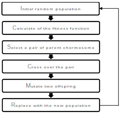
The GA was developed by [55] who defined the VRPTW solution code in the form of bit strings or chromosomes. The objective of the GA algorithm is to find the fitness function by using a set of parameters, which are population size, crossover rate to create new children, and random mutation rate [56]. stated that a population size between 50 and 100 is the best for generating a solution [57]. mentioned that the crossover rate and mutation rate are the two important factors for the reproductive process in GA. A crossover rate ranging between 0.6 to 0.9 gives a higher chance of producing an offspring [58]. However, mutation is used to prevent the situation where all of the chromosomes in the initial population have the same value at a particular position because it leads to having the same value for the future offspring. The mutation rate is suggested to be low, which ranges from 0.005 to 0.01 [59]. The process of GA is detailed as shown in Fig. (1).
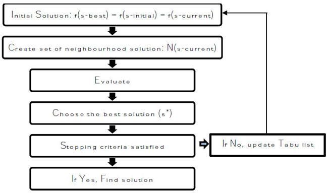
The TS is a methodology that uses a memory-based search to direct the local search to keep searching for a local optimal solution [60, 61] indicated that the use of the Tabu list is comparable to human memory, which prevents the moves from revisiting the local optimum on the Tabu list. Furthermore, the Tabu search also allows non-improving moves to search the solution, which is beyond local optimal solutions. TS is the most effective in solving a large number of problems to get close to the optimal solution and will stop after a fixed emphasis number. TS uses a neighbourhood to move and choose the move to compose the best of all solutions. The TS has a clear memory component. The purpose of using the TS for the VRP with measurements is to help both the recency-based memory (short-term memory) and frequency-based memory (long-term memory) [60]. Although many researchers, such as [62, 63], have used the TS to solve the VRP, few researchers have used it to solve the VRPTW [64]. used the TS algorithm on the VRPTW, which changed the objective from the normal VRP to minimise the total cost or distance, to reduce the number of vehicles. The process of TS is shown in Fig. (2).
3. PROBLEM ANALYSIS AND MODELLING
3.1. Problem Description
The general assumption in the VRP is that vehicle speed could be constant and traffic congestion commonly causes certain road conditions based on time-dependence. However, the speed of a vehicle cannot be constant all the time and, in fact, it is constantly changing due to traffic conditions and different roads. In this study, the researcher considered time-dependence for vehicle routing and multiple time periods for vehicle scheduling with the main objective being to minimise the travelling distance, the operation cost in terms of fuel consumption, and CO2 emission considerations. This work also studied the optimisation of the fuel emissions in a travelling route where a vehicle’s speed depends on time, a fixed location of the customers under the company’s responsibility, and the number of vehicles available for delivery of the goods is limited.
3.2. Modelling
The TDPRP has been explained on a complete graph, G = {N, A}, where N was a set of customers, 0 was the depot, and A was the set of arcs between every customer. The distance between customers was denoted by dij, where i ≠ j. There was a homogeneous fleet of K vehicles in which each truck had a capacity limit of Q units and all the vehicles had to begin and end at the depot. Each customer demand, qi, had to be delivered by one truck. The service time was Si and the time window [li,ui] of each customer was considered. In particular, if a vehicle arrived at customer i before li, it would wait until time li started to service, without loss. And, also a vehicle had to arrive at customer i before ui in order to load the product. We assumed that the vehicle could leave from the depot and get back to the depot within the time window.
3.3. Time - Dependency
[49] Bektaş and Laporte (2011) stated that the travelling time of each arc depends on the distance and vehicle speed. In this project, the vehicle speed also depended on the time period that the vehicle would leave from the last node because there were different maximum speeds for each time period. The traffic time was divided into 3 time periods, starting from a free-flow period to a congestion period and ending with a free-flow period, respectively. The vehicle speed on the road traffic was expected to be fixed within a time period, but could have been different between each time period, as shown in Table (1).
| Time Period | Average Vehicle Speed |
|---|---|
| 1:00 – 5:30 (Free-Flow) | 60 Km/Hr |
| 5:30 – 10:00 (Congestion) | 30 Km/Hr |
| 10:00 – 12: 00 (Free-Flow) | 60 Km/Hr |
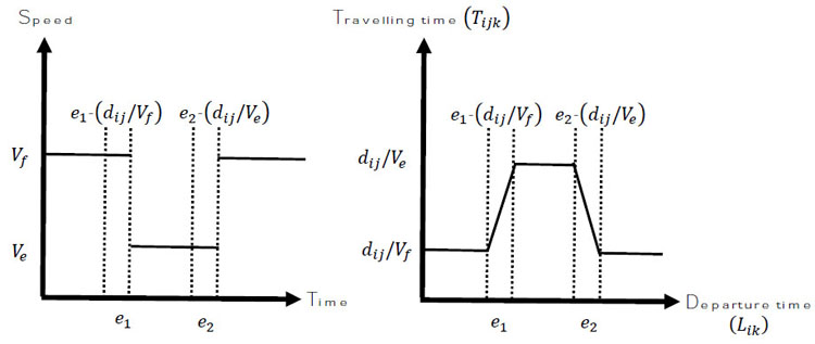
Let T represent the set of time periods, each period t  T, and it is identified by beginning time bt and ending time et. The vehicle speed in the congested time and free-flow are denoted by vc and vf. Tijk denotes the travelling time of a vehicle between customers, which spent time by vehicle k on the arc (i,j), depending on departure time Lik from node i, and the vehicle speed in different time periods. The formulation used for calculating the travelling time in (1) was adapted from the original formulation proposed by [51]. The relationships between the departure time and speed & departure time and travelling time are shown in Fig. (3).
3.4. Modelling Emissions
The modelling of emissions and fuel consumption have been described by [49] in their discussion on topic of “Pollution Routing Problem”. The approach for an emission model shows that GHG emissions are directly converted from the fuel consumption. This approach called the “comprehensive emission model” was first presented by [4, 65]. However, it was a very complex formulation so [49] simplified the original approach. By following [49] approach, we needed to find the total energy used over an arc (i,j) and then convert it into fuel consumption and GHG emissions, respectively. For the Energy-based approach by Guidelines for Measuring and Managing CO2 Emissions from [66], it indicates that the easiest and most accurate way for transportation companies to calculate transportation emissions is to use the total fuel consumption and emission conversion factors to convert energy or fuel values into CO2 emissions.
The equation to calculate CO2 emissions is shown below: CO2 emissions = fuel consumption x fuel emission conversion factor. However, it is very important for the hauler to use the correct emission conversion factor for the different types of fuel being used, as shown in Table (2). We know the fuel emission conversion factor in different types of fuel, but fuel consumption, F, needed to be found. Calculation of F is complex, thus the equation for calculating F provided by [65] was used.
4. METHODS
4.1. Data Collection
The project needed to simulate the situation from the accurate data of a logistics company in Thailand providing the services of local delivery, drayage, cargo tracking, and EDI support. To provide the best logistics solution, service, and support to its customers under the traffic problem in Bangkok, this company had been chosen in this study. This company started running its business in the year 2000; it has been running it for over 18 years. The company has operated a domestic business, which is one of the largest logistics providers in Thailand. It also includes providing consultancy of the integrated Third-Party Logistics, as well as becoming long-term business partners with globally integrated logistics management companies. With 300 plus manpower, it effectively delivers the quality and standardised service to satisfy its customer’s needs and has different types of transportation vehicles, such as 4 wheels, 6 wheels, 10 wheels, and 18 wheels. In addition, to ensure that the model was constructed accurately, the data was collected from the staff to make sure that the data was up-to-date. Moreover, some information was collected by interviewing the owner of the company. The data given by the company was used in the model testing in combination with the data collected from journals and the internet such as the distance between customers, traffic time period, maximum speed of vehicle at different traffic time, emission rate, etc.
| Fuel Type | kg CO2/liter | kg CO2/kg |
|---|---|---|
| Motor Gasoline | 2.8 | – |
| Diesel Oil | 2.9 | – |
| Gas Oil | 2.9 | – |
| Liquefied Petroleum Gas (LPG) | 1.9 | – |
| Compressed Natural Gas (CNG) | – | 3.3 |
| Jet Kerosene | – | 3.5 |
| Residual Fuel Oil | – | 3.5 |
| Biogasoline | 1.8 | – |
| Biodiesel | 1.9 | – |
4.2. Model Implementation
Before calculating the CO2 emissions, there were many other parameters and constraints needed to be known, for example, the optimal route for each vehicle, travelling time, distance between a pair of customers, energy consumed for each route, capacity constraint, time window constraint, etc. First of all, all of the data needed to be defined because it was to be used in other processes of calculations. The data that are defined including customer ID, customer order, time window of each customer, and distance between customers i to j.
Parameters include allocating customers for vehicles, distance calculation, and defining vehicle speed and travelling time calculation. Firstly, to allocate customers for vehicles, a summation of customer’s demand in one route must not exceed the maximum load (60 baskets per each vehicle). The customer’s ID is a decision variable of this model. Therefore, all the calculations are dependent on these values. After the customer orders are known, the next value needed to find is the accumulation of the customer orders, called delivered baskets. It can be calculated by the summation of previous customer’s orders plus the current customer’s order and if it exceeds 60, it means the customer will be assigned to another route. Secondly, it is moved to the route table because the start and endpoint, which is the depot, is not included in the previous step. The distance from the previous location to the current location can be known by using the following formula: =INDEX (Distance, previous location, current location). Thirdly, the parameters of Defining vehicle speed and travelling time calculation depend on the departure time from the last node because there are different maximum speeds for each time period. Before calculating the travelling time, it needs to know at what speed the vehicle uses to transport along the arc of two customers.
The solution of this model is to minimise the total CO2 emission that a company generates during the day in the transport process. If a company runs a business with 9 vehicles, this means there are 9 routes for delivering products to customers. The total CO2 emission that a company generates during the day can be calculated by a sum of CO2 emission emitted in each route.
5. RESULTS AND DISCUSSION
There were two algorithms used in this research, which were the Genetic Algorithm (GA) and Tabu Search (TS), as the solution methods. For the Genetic Algorithm, the initial population size, crossover operator, and mutation operator were set at a specific value to generate the best solution as was mentioned in the literature. The Tabu Search (TS) was used in OptQuest. Both methods had a stopping condition as a certain number of trials. Finally, the results of both methods were compared in terms of computation time and solution. Moreover, the best solution was compared with the current solution of the company in order to show the improvement.
5.1. Genetic Algorithm
In order to generate the optimal solution, all constraints were considered, including the vehicle capacity constraint, customer’s time window constraint, and time-dependency constraint related to the congestion time period. Moreover, all the vehicles had to begin and end at the depot and all the customers were visited only once. The evolver was set with the following settings: Population Size (50), Crossover Rate (0.9), Mutation Rate (0.01), and the stopping criteria were set at 10,000 and 30,000 trials.
The combination used the crossover rate of 0.9 and mutation rate of 0.01 to generate the solutions. The best solution was found at 0:02:41 within a total optimisation time of 0:02:42 and the stopping criterion was at 10,000 generations. The original solution was 320.9427. By using the combination, the minimum CO2 was reduced to 215.7832. In contrast, the routing of the initial solution was different from the routing of this combination. In addition, the best solution was found at 0:03:43 within a total optimisation time of 0:08:28 and the stopping criterion was at 30,000 generations. The original solution was 320.9427 but it was reduced to 190.9277 by using the combination. In comparison, the routing of the initial solution was different from the routing of this combination.
5.2. Tabu Search
First of all, the constraints could not be exceeded. There were three hard constraints, which were the vehicle capacity constraint, customer’s time window constraint, and time-dependency constraint related to the congestion time period. Moreover, all of the vehicles had to begin and end at the depot and all the customers were visited only once. The evolver was set to use the manual optimisation mode, and the optimisation was achieved using OptQuest as the Tabu Search method. The stopping criteria were set at 10,000 and 30,000 trials.
For optimisation using OptQuest as the Tabu Search Method, the best solution was found at 0:35:59 within the total optimisation time of 0:36:03 and the stopping criterion was at 10,000 generations. The original solution was 320.9427. Whilst the minimum CO2 emissions using OptQuest were reduced to 198.3520. Contrary to that, the routing of the initial solution was different from the routing from this optimal solution. In addition, the best solution was found at 2:19:37 within the total optimisation time of 2:28:20 and the stopping criterion was at 30,000 generations. The calculated solution using the combination was 183.9846 whilst the original solution was 320.9427. In contrast, the routing of the initial solution waa different from the routing from this optimised solution.
5.3. Comparison of the Results and Computation Times
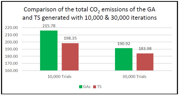
As a result, all the solutions of both algorithms, which were the Genetic Algorithm (GA) and Tabu Search (TS) needed to be compared in terms of the quality of the solution and computation time. Furthermore, the model was run with the stopping criteria at 10,000 iterations and 30,000 iterations from the initial solution, it was clear to see that the TS method gave a better solution than the GA method in both cases, which were stopping conditions at 10,000 trials and 30,000 trials. As shown in Fig. (4), the total CO2 emissions using 10,000 trials as a stopping criterion to generate the solution for the GA method and the TS method were 215.78 kilograms and 198.35 kilograms, respectively.
Similarly, when 30,000 trials were used as a stopping criterion, the total CO2 emissions generated by the GA method were 190.92 kilograms and the solution of 183.98 kilograms was generated by the TS method. On the other hand, the computation times that the GA method used to generate the solution were faster than with the TS method, based on the comparison depicted in Fig. (5).
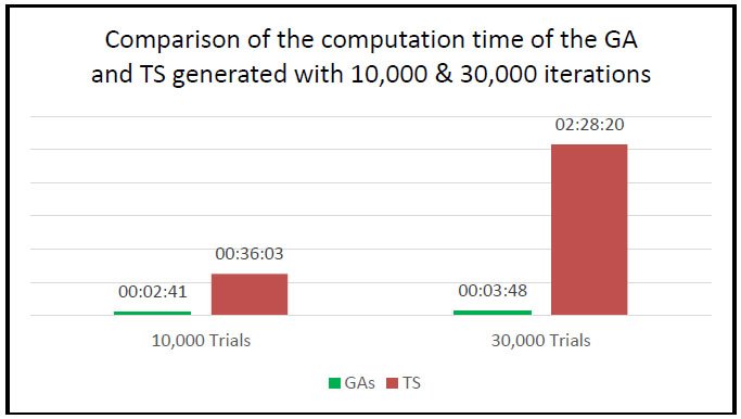
The GA method took a few minutes to find the best solution. However, the TS method took a lot more time for optimisation and the computation time increased as the number of iterations increased. Fig. (3) showed the computation time of both the GA and TS; generating solutions using the TS method with 10,000 trials took 36:03 minutes and it dramatically increased to 2:28:20 hours as the number of trials increased to 30,000 trials. The convergence plot is shown in Fig. (6).

5.4. The Best Solution for the Model
The best solution was generated by using the TS method with 30,000 trials. The minimum of the total CO2 emissions was 183.9846 kilograms produced from all of the vehicles during transportation. When compared with the current transportation plan of the company, it generated 320.94 kilograms of CO2 emissions. It is clear to see that almost half of the CO2 emissions were reduced. In other words, the model could help the company to improve its transportation plan because the CO2 amount was proportional to the distance. This is because the new transportation plan uses only eight vehicles to deliver products to all the customers, despite the original transportation plan used nine vehicles. Moreover, the model also rearranged the order of the customers for each vehicle in order to minimise the distance. On top of this minimisation, the operation costs of the company, including fuel cost and driver cost, were reduced. However, a better solution could be found in this model by adding more iterations and using the TS method for optimisation.
Based on the above analysis, all of the data was collected from the logistics company providing a service in Bangkok, Thailand. There were essential information factors related to the conditions used for building the model. The results show that: (1) The performance of the GA and TS for solving congestion and pollution VRPs are different in their own characteristics due to the differences in the algorithms. The TS algorithm performed well in terms of the quality of the solution and stability; as [66-69], mentioned that TS approaches have an average deviation of 0.5% - 1%. On the other hand, the GA provided a very fast computation time. (2) The shortest route based on the minimal total costs and CO2 emissions were generated by the TS. In this study, the optimal transportation plan reduced CO2 emissions by 50% compared with the previous transportation plan. (3) The new transportation model reduced the number of vehicles from nine vehicles to eight vehicles for the delivery of the goods, by which it could reduce the operation costs compared with the previous travel route plan.
CONCLUSION
This paper studied a time-dependent and pollution vehicle routing problem model, where a number of vehicles served the customers to minimise CO2 emissions and operations costs. The important factor was traffic congestion as it directly affected the vehicle speed where the CO2 emission rate also depended on the vehicle speed and vehicle load. The implemented model optimised both the route and schedules (multiple time periods) for a number of vehicles, for which the transportation during a fixed congestion period could be predicted to avoid traffic congestion and reduce the CO2 emission. In this study, meta-heuristics methods were utilised in the proposed approaches to minimise the congestion and pollution VRP. The performance of the GA and TS algorithms was able to solve the VRP, which were different in their own characteristics. The Tabu Search algorithm resulted in a better solution than the GA in terms of quality and stability. Except, the computation time had taken longer than with the GA. However, the proposed transportation model and method can be used to minimise the operation costs and CO2 emissions for the logistics companies.
Based on the results, the logistics firms should use the proposed transportation model and method to reduce the companies’ operational costs and save the environment. This will lead to the companies providing their customers with the best logistics solutions, services, and support. For future research, there is a need to enhance the model with higher accuracy of fuel consumption and emissions by considering many other specific parameters, such as an adaptive large neighborhood search heuristic for pollution-routing problems [68]. Green Vehicle Routing Problems (GVRP) [69]: routing light delivery vehicles using a neuro-fuzzy model [70], artificial search agents with cognitive intelligence [71], swarm intelligence based algorithms for the set-union knapsack problem [72]. In addition, there are other constraints that are not measured in the model. As in the real world, transportation problems are much more complex than just 2-3 constraints. Therefore, the model allows for the addition of other constraints in order to make the model more realistic.
CONSENT FOR PUBLICATION
Not applicable.
FUNDING
None.
CONFLICT OF INTEREST
The author declares no conflict of interest, financial or otherwise.
ACKNOWLEDGEMENTS
Declared none.

