All published articles of this journal are available on ScienceDirect.

Using Generalized Linear Mixed Models to Predict the Number of Roadway Accidents: A Case Study in Hamilton County, Tennessee
Abstract
Introduction:
A method for identifying significant predictors of roadway accident counts has been presented. This process is applied to real-world accident data collected from roadways in Hamilton County, TN.
Methods:
In preprocessing, an aggregation procedure based on segmenting roadways into fixed lengths has been introduced, and then accident counts within each segment have been observed according to predefined weather conditions. Based on the physical roadway characteristics associated with each individual accident record, a collection of roadway features is assigned to each segment. A mixed-effects Negative Binomial regression form is assumed to approximate the relationship between accident counts and several explanatory variables including roadway characteristics, weather conditions, and several interactions between them. Standard diagnostics and a validation procedure show that our model form is properly specified and suitably fits the data.
Results:
Interpreting interaction terms leads to the follow findings: 1) rural roads with cloudy conditions are associated with relative increases in accident frequency; 2) lower/moderate AADT and rainy weather are associated with relative decreases in accident frequency, while high AADT and rain are associated with relative increases in accident frequency; 3) higher AADT and wider pavements are associated with relative increases in accident frequency; and 4) higher speed limits in residential areas are associated with relative increases in accident frequency.
Conclusion:
Results illustrate the complicated relationship between accident frequency and both roadway features and weather. Therefore, it is not sufficient to observe the effects of weather and roadway features independently as these variables interact with one another.
1. INTRODUCTION
Roadways in the United States are among the busiest in the world, with more than 240 million vehicles registered and more than 210 million registered drivers [1]. With such busy roadways, we naturally see a high number of motor vehicle accidents. According to the US Department of Transportation and the National Highway Traffic Safety Administration, there were over 7 million motor vehicle crashes in 2016 on US road ways [2]. With these accidents come serious costs to Americans. According to 2015 statistics, motor vehicle crashes were the leading cause of death in the first three decades of Americans’ lives [3]. Furthermore, roadway accidents are responsible for $77.4 billion in loss of productivity, $76.1 billion in property damage, $31.5 billion in congestion/delay, and $23.4 billion in medical costs [4].
While roadway crashes are an unavoidable consequence of busy roadways, researchers in the field aim to find ways to mitigate roadway accidents. To this end, we ask: “why do some roadways observe more accidents than others?” If we can identify the factors or conditions most closely associated with roadway accidents, then our findings may inform transportation administrators of the nature of roadway crashes, ultimately helping these decision-makers to implement policy changes to improve safety.
The primary objective of this work is to find the roadway characteristics, weather conditions, and potential interactions between roadway characteristics and weather conditions associated with the variability in observed accident counts. This will be achieved via a Negative Binomial regression model that identifies relationships between accident counts and combinations of weather conditions and roadway features. We feel this approach is novel in that it 1) combines diverse sources of data, weather and roadway characteristics, that are critically important to explaining accident frequency, and 2) uses a flexible model structure that allows us to consider both random effects as well as a variety of interactions between variables that may potentially shed light on the complicated nature of accidents. To the best of our knowledge, currently, no work uses a mixed-model in conjunction with combinations of weather and roadway features. As an application, we consider real-world accident data collected from Hamilton County, Tennessee. Hamilton County is an ideal location for a case study as it contains busy, metropolitan areas surrounding Chattanooga (Tennessee’s fourth largest city) as well as a number of residential and rural areas. As such, the county has a variety of roadway types (from major interstate highways to rural backroads) and our results are likely to be transferable/generalized.
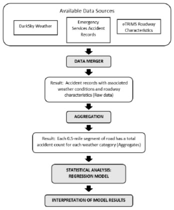
The remainder of this paper is organized as follows: Section 2 (Literature Review) presents previous research related to this work; Section 3 (Data and Preprocessing) presents the available data used in the analysis, how these data sources are merged together, and ultimately how the data are aggregated into accident counts for each roadway segment; Section 4 (Statistical Modeling) presents the statistical model to be used in this analysis and the theoretical justification for the model choice; Section 5 (Model-fitting) discusses details of the model-fitting procedure and further justification of the model; Section 6 (Results) presents interpretation of model-fitting results as well as diagnostic tests for the model; Section 7 (Validation) provides evidence that our model specification is appropriate for the data; and Section 8 (Discussion and Conclusion) provides a summary of the procedure, potential application, and potential refinements for future studies. As this work involves a complicated process using multiple sources of data and substantial data preparation, a workflow of the analysis is presented below in Fig. (1) to assist the reader.
2. LITERATURE REVIEW
As stated above, our work uses a regression model to identify relationships between accident frequency and combinations of weather conditions and roadway features. Previous research has shown that many roadway features, particularly those available to us, are strongly associated with roadway accidents. Specifically, AADT/DHV/ traffic volume [5-7], roadway type [8], terrain/grade [9-11], land use /type of road/urban versus rural roadways [12, 13], illumination [9], posted speed limit [9, 14, 15], pavement widths [11, 16], pavement type [17], presence of on-ramps/off-ramps [18-20], and number of lanes [10, 12, 21], have all been linked to roadway accidents.
In addition to roadway features, weather conditions have been shown to play a role in explaining the variability of accident counts. In an analysis of accident frequencies in Great Britain, Edwards [22] presented temporal trends for 9 broad weather categories as defined by the Department of Transport. More generally, other works suggest weather conditions, especially precipitation events, are important components of accident prediction [18, 20, 23-29], and we know intuitively, as drivers, that roadways become more dangerous in inclement weather.
For this analysis, we use a mixed-effects Negative Binomial (NB) model. There is extensive literature supporting the use of the NB form to model roadway accidents, yet these works vary considerably in terms of scope. Chengye and Ranjitkar [20] used NB models and data collected from a motorway in Auckland, NZ to link accident frequency to ‘non-behavioral’ factors such as traffic conditions, roadway characteristics, and weather conditions. The authors performed three NB analyses: one on the entire motorway, one separating urban and rural sections, and one separating segments by on- and off-ramps. Shankar et al. [26] used a NB model on data collected from rural highways to identify relationships between accident frequency and roadway geometry, weather factors, and various interactions between them. Hall and Tarko [30] showed that the NB form was suitable to model accident frequency on low-volume, rural roads. Milton and Mannering used the NB model and data collected from Washington highways to isolated the effects of geometric and traffic characteristics on annual accident frequency [31]. Abdel-Aty and Radwan [21] used the NB form to model the frequency of Florida highway accident occurrence based on roadway geometry, urban/rural designations, and section length (the authors also developed NB models to account for age and gender of the driver). Eisenberg [27] used both monthly and daily precipitation as explanatory variables, and found a negative correlation between monthly precipitation and fatal accidents. Chin and Quddus [32] used a random-effect NB model on data collected from signalized intersections in Singapore to identify relationships between accident occurrence and the geometric, traffic, and control characteristics. Shankar et al. explored NB and random-effect NB forms to model median crossover accident frequencies for several routes in Washington [33]. Using roadway geometry, traffic volume, and a random effect to account for different routes, they found the random-effect model to be superior [33]. In a related study, Ulfarsson and Shankar used the same explanatory variables to compare NB and random-effects NB models to a Negative Multinomial model form for accident frequency [34].
As seen, there are numerous works using the NB regression form and/or random-effects models to approximate roadway accidents, and there are works that consider roadway features and/or weather conditions in their statistical models. However, to our knowledge, no current work exists that implements both a random-effect model and this combination of roadway characteristics/features and weather conditions, including interactions between them. Herein lies the novelty of our work.
3. DATA AND PREPROCESSING
3.1. Available Data
A hallmark of this work is the use of detailed and accurate datasets from three distinct sources: Hamilton County emergency services, eTRIMS, and DarkSky.
3.1.1. Hamilton County Emergency Services
The Hamilton County Emergency Communications Center provides emergency dispatch service for 105 Police, Fire, and EMS departments covering 42 political jurisdictions in the county. This service, which collects reports from first responders, was used to collect information for traffic accidents in Hamilton County between January 1, 2017 and December 31, 2018 (the collection period). Importantly, each accident record has an associated physical location measured in terms of route mile marker (log-mile).
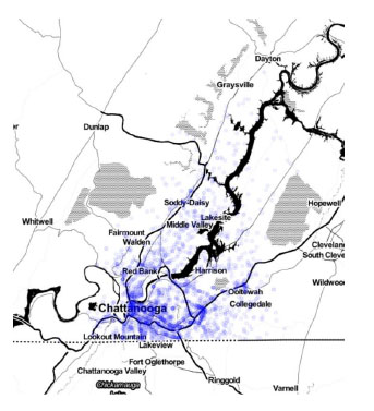
Over the collection period of two years, 55,324 total accidents were reported in Hamilton County. As seen in Fig. (2), accidents occurred in highly populated areas within the city limits of Chattanooga as well as in less populated, rural areas in the county.
3.1.2. eTRIMS
Since the 1970s, the Tennessee Department of Transportation (TDOT) has maintained location descriptions and inventory data on all local roads. This information was integrated into the Tennessee Roadway Information Management System (TRIMS) that serves as a referencing database for State and local roadway information. In 2007, TDOT began developing eTRIMS, a map-centric, web-based version of TRIMS with the purpose of encouraging wider use of the TRIMS database. Based on previous literature (Literature Review) and the data available for Hamilton County via eTRIMS, we consider the following roadway and pavement characteristics for our analysis.
- Average Annual Daily Traffic or AADT (numerical variable)
- Administrative System (categorical variable representing road system designation; i.e., city highway, city road, interstate, rural highway, or rural road)
- Terrain (categorical variable; i.e., flat, rolling, mountainous)
- Land Use (categorical variable representing designation of the surrounding land; i.e., commercial, industrial, public, residential, rural, or a combination)
- Illumination (indicator variable designating if street lamps are present)
- Posted Speed Limit (numerical variable, measured in miles per hour)
- Pavement Width (numerical variable, measured in feet)
- Pavement Type (categorical variable; i.e., asphalt, cement)
- Design Hour Volume or DHV (numerical variable)
- Number of Lanes (numerical variable)
- Presence of on- and off-ramps (indicator variable)
Since accident records have precise log-mile locations (a designation amenable to the eTRIMS database), the roadway characteristics listed above are easily assigned to each of these accident records.
3.1.3. DarkSky Weather
DarkSky [35] is an API for Python that collects weather data from several weather resources and makes available information associated with specified locations at precise time periods. Since our accident records have both a time and latitude/longitude designation (designations amenable to the DarkSky data), Darksky weather conditions are easily assigned to each.
For our analysis, to assist the model-fitting procedure and make results more interpretable, we simplify the available weather information. Specifically, we consider a continuous variable for visibility (measured in miles) and a categorical variable that distinguishes between the following broad weather categories.
- Clear - no precipitation, no clouds
- Start rain - currently raining, no rain in the previous time step
- Continue rain - currently raining, raining in previous time step
- Start cloudy - currently cloudy, not raining/cloudy in previous time step
- Continue cloudy - currently cloudy, raining in previous time step
- Fog
In their study of the effects of weather on accident risk, Malin et al. [23] used similar, discretized categories for weather conditions.
3.2. Descriptive/Summary Statistics of Data
| Weather Condition | No. Accidents | % Total |
|---|---|---|
| Start cloudy | 34,447 | 62% |
| Clear | 10,667 | 19% |
| Start rain | 4,355 | 8% |
| Continued cloudy | 2,707 | 5% |
| Continued rain | 1,842 | 3% |
| Fog | 1,283 | 2% |
| Other (including missing) | 23 | .04% |
| Rd. Type (Admin. Sys.) | No. Accidents | % Total |
|---|---|---|
| City road | 33,120 | 60% |
| City highway | 11,515 | 21% |
| Interstate highway | 8,073 | 15% |
| Rural road | 1,958 | 4% |
| Other (including missing) | 490 | 1% |
| Rural highway | 168 | .3% |
3.3. Combining Data/Creating Roadway Aggregates
3.3.1. Defining Roadway Segments
We observe roadways in terms of short, non-overlapping segments. This serves two purposes. First, segments act as interval in which to collect counts, since it is unlikely that more than one accident would occur at any one precise location. Second, by setting the segments to some short, fixed lengths, we are defining a fine gradient over which we view our roadways. Then, by observing roadway features associated with accidents within these short segments, we aim to capture the heterogeneity/variability of roadways (Table 1).
Our choice of segment length is based on the level of precision used by traffic engineers when observing roadways. Traditionally, actual locations on a roadway, or ‘spots,’ are lengths greater than 0.1 miles as this is believed to be a minimum threshold to discern differences in locations [36]. Others have suggested spot lengths to be at least 0.3 miles long [37] or between 0.3 and 0.5 miles [36]. Segments, then, should be longer than spot distances. With the aim of capturing as much variability in roadway characteristics as possible, we set our segment length at the upper limit for spot length, and we thus define segments as half-mile sections of roadways. Note: subsequent results varied little when choosing segments of slightly shorter (0.3 and 0.4 miles) or longer length (0.6 miles).
For simplicity, our segment length is held constant (fixed-length segmentation) for all roadways in the collection area. Certainly, there are more complicated approaches to identifying roadway segments (many of which are beyond the scope of this analysis); such as those defining segments based on changes in AADT [38], curvature and roadside danger [39], or a variety of roadway geometries [40]; but there is no universally agreed-upon approach. In their comparison of the effect of roadway segmentation criteria on the performance of safety performance functions, Cafiso et al. [7] found that fixed-length segmentation (such as we have) was a flexible and statistically consistent technique. Also, in their study focusing on the relationship between crashes, road geometry, and segmentation, Cenek et al. [41] used fixed-length segments (Table 2).
3.3.2. Creating Aggregates
Aggregation, in our case, involves combing accident data, roadway characteristics, and weather conditions for each of the half-mile segments across the county. This task is conceptually straight-forward since all accident records have been previously linked to corresponding roadway characteristics and weather conditions, and each has a log-mile designation.
Note: As we do not want to average weather within segments (and potentially wash away any weather signal), for each segment we create an accident count for each weather category. This allows us to introduce the weather as an explanatory variable in our regression model.
Note: For continuous roadway features (AADT, for example), each segment is assigned the average of values associated with accidents in that segment. For categorical features (terrain, for example), the most commonly observed value is assigned to each segment. Lastly, two features are measured in terms of presence/absence: illumination and change in a number of lanes. Since most segments were homogenous in terms of illumination, we identify a segment as having illumination if most observations had that designation. For the presence of a change in the number of lanes, since we believe the effects of exiting/entering/merging/weaving extend beyond the locations where change occurs, we designate a segment as having this feature if any of the records in the segment had this feature (Table 3).
3.3.3. Final Comments Regarding Segments/Aggregates
After some data cleansing to remove incomplete records, we were left with 5,505 aggregated segments, which will provide the basis for our model-fitting procedure. For each of these, we retain the original route identification to be used as a random effect, or to account for potential roadway variation (literature supports the need for such a designation; see, for example, [15, 42, 43]. Lastly, we note that the segment/ aggregate will not be used in our modeling procedure as accident count variability between aggregates is believed to be attributable to segment/aggregate characteristics, weather, or some combination of the two. Also, in an initial data investigation, no autocorrelation was found to exist between counts from adjacent segments/aggregates.
4. Statistical Modeling
For our data, we initially pursued a Poisson regression model to approximate our accident counts by roadway segment. Such models are theoretically justified as they are designed to model count data. A somewhat restrictive drawback of this model, however, is the Poisson assumption of equi-dispersion (equality of mean and variance). In our case, an initial investigation of the data revealed our count data is over-dispersed (thus, not equi-dispersed) and thus does not follow a Poisson distribution. For such cases, to model count data that does not necessarily follow a Poisson distribution, the Negative Binomial regression model form is typically recommended as a remedial measure. The Negative Binomial model form is considered a variant of the Poisson form and includes an additional parameter to account for over-dispersion. Also, as there is likely a roadway-specific effect on the accident counts, or rather a natural heterogeneity between accident counts collected at different routes, we introduce a random effect component for the roadway. As stated by Ulfarsson and Shankar [34], in the case of accident frequency, it is likely that section-specific effects will be important. Our model is:
| Roadway Characteristic | No. Accidents | % Total |
|---|---|---|
| Land Use | ||
| Commercial | 21,455 | 39% |
| Residential | 14,306 | 26% |
| Rural | 12,298 | 22% |
| Industrial | 1,472 | 3% |
| Other | 5,793 | 10% |
| AADT | ||
| <50,000 | 43,034 | 78% |
| ≥50,000 | 12,290 | 22% |
| Posted Speed Limit | ||
| ≥60 | 2,494 | 5% |
| [50, 60) | 9,111 | 16% |
| [40, 50) | 14,722 | 27% |
| [30, 40) | 15,840 | 29% |
| <30 | 2,948 | 5% |
| missing | 10,209 | 18% |
| Pavement Width | ||
| <8 ft. | 27,469 | 50% |
| ≥8 ft. | 27,769 | 50% |
 |
with α the NB dispersion parameter, and
 |
where yij is the accident count from the ith segment of the jth roadway, uj is the random effect for the jth roadway, β is the vector of fixed-effects model parameters, xi,j is the design-vector for the ith segment of the jth roadway, and u~N(0,σ2).
Very often, count-based regression models like the Negative Binomial include an ‘offset variable’ to account for disparate ‘exposures’ in the data. A common source of varying exposures is changes in collection periods. This, however, is not the case with our data. That is, our data consist of all roadway accidents reported in the county for a two-year period, so each record represents the total number of accidents occurring in that segment over that two-year period. On the other hand, our data does consist of very diverse roadways that experience varying degrees (exposures) of travel and volume. Thus, an argument could be made to use AADT, a measure of traffic volume, as an offset. We have decided against using AADT (or any other measure of traffic volume, demand, etc.), however, as we wish to directly quantify the relationship between AADT and accident totals, an analysis that would not be possible if we use it as an offset. In their analysis of crashes caused by the running of red lights using Poisson and NB models, Mohamedshah et al. [44] similarly omitted AADT as an exposure/offset variable. In the end, no offset was used in our model.
5. MODEL-FITTING
All model-fitting and statistical analyses were performed using the R statistical software system [45]. In addition to the base packages in R, the ‘lme4’ and ‘MASS’ packages [46, 47] were used extensively. Model-fitting was performed via maximum likelihood estimation.
5.1. Independent/Dependent Variables
For our model, we define the response/dependent variable to be the accident count. For the independent variables, we consider fixed-effect terms for average AADT, average speed limit, average pavement width, average DHV, average visibility, average number of lanes, most occurring administrative system, most occurring terrain, most occurring land use, most occurring pavement type, the presence/absence of illumination, and the presence/absence of change in number of lanes; a fixed-effect, categorical term to distinguish accident counts observed under different weather conditions; and a random-effect term for the different roadways (routes). Also, since we assume that the relationship between roadway features/weather and accident frequency is potentially complicated, several logical interactions will be considered. Related to this, in their analysis of safety performance functions, Islam et al. [48] identified the importance of incorporating interactions between variables (in particular, those between speed limit and geometric variables) for estimation of crash prediction models.
5.2. Justification for Model Specification/Preliminary Analyses
Since the Poisson model form is nested within the NB model form (the NB model has one additional parameter to account for the over-dispersion), we performed a likelihood ratio test to assess whether or not the use of the more complicated model, the NB model, is justified. As suspected, we found that the NB model form provided a statistically significant improvement over a comparable Poisson model (Likelihood ratio X2= 27002, df = 1, p-value < 0.0001). Thus, the NB model form was has pursued for this analysis.
Next, to assess if the inclusion of a random effect is necessary, we compared our NB model form with a simpler NB form with only the fixed effects. As above, the models were compared via likelihood ratio test, and it was found that the NB model with a random effect for the route was a statistically significant improvement over the NB model without the random effect (Likelihood ratio X2= 1198, df = 1, p-value < 0.0001).. Thus, the random intercept term was retained for all future analyses.
Finally, we investigated potential multicollinearity between the explanatory variables since severe multicollinearity can result in coefficient estimates that are unstable and difficult to interpret. Using the ‘car’ package in R [49], because we have a combination of continuous and categorical variables, we calculated the Generalized Variance Inflation Factors (GVIFs) for our NB model with only main effects and a random-effect for the route. None of the squared GVIF
 quantities [50] are larger than 4, suggesting that multicollinearity is not an issue with this set of explanatory variables. Although we expected average AADT and an average number of lanes to be related, for example, the correlation between them does not appear to be troublesome. Also, for these two variables specifically, a likelihood ratio test indicated that both variables should be included in the model (Likelihood ratio X2= 116.36, df = 1, p-value < 0.0001).
6. RESULTS
6.1. Initial Results
Using the ‘MuMIn’ package in R [51], we calculate the conditional pseudo-R-squared or an estimate of the percentage of the observed variance in the response explained by the mixed-effects model. For our best model, we have a pseudo-R-squared of about 0.80 (0.7959), an indication that our model is highly successful in explaining the variability observed in our accident frequencies. In their NB analysis of accidents on roadway segments with on-ramps, Chengwe and Ranjitkar [20] achieved a likelihood ratio index (somewhat comparable to R-squared) of about 0.19. In their analysis of the frequency of accidents at intersection approaches, Poch and Mannering [52] used several NB models on different types of accidents, and their best model achieved a likelihood ratio index around 0.54.
6.2. Interpretation of Parameter Estimates
For several reasons, interpreting the results of our fitted model is not straight-forward. First, since we assume an NB form, our explanatory variables have a log-linear relationship with our response variable. This means that our estimated parameters must be ‘exponentiated’ to assess their relative effect on the response variable (that is, calculate an ‘incidence rate ratio’). Second, as recommended by Bates et al. [46], our continuous explanatory variables were scaled to facilitate the convergence of our model. Thus, these variables are converted to standard deviation units from their mean values (this means continuous variables can have negative values which correspond to values less than the average). Third, we consider a variety of interactions, so relationships between explanatory variables and the response become more complicated and nuanced. Fourth, we have a number of categorical variables, and results for those variables are presented as changes from the ‘base case’ category. Lastly, we have a large number of variables and interactions and it is not reasonable to present and interpret all parameter estimates. However, in the following sub-sections, we will discuss several estimates that are statistically significant and noteworthy.
Note: a beneficial byproduct of centering variables is that, for some cases, it allows for interpretation of main effects when an interaction is present. Typically, the main effects are not interpreted in the presence of interaction since, in such cases, the main effect represents the effect of one variable when the other is set at a value of zero. This is often an unrealistic scenario as it would be unlikely to observe a variable at a value of zero. However, for centered variables, zero now represents the average, which is realistic.
6.2.1. Administrative System (Roadway Type) and Weather
From the analysis of variance of our best-fitted model, we find that the interaction between administrative system and weather condition (both categorical variables) to be very significant (Type II Wald Chi-square test, X2 = 91.2118, d.f. = 22, p-value = 2.130e-10). Among the specific levels of these two variables, we find the parameter estimate associated with the interaction between “rural road” type and the “start cloudy” weather condition to be significant.
Table (4) below gives the regression model output associated with these variables.
| Variable | Regression coefficient | Tests statistic (Wald Z value) | p-value |
|---|---|---|---|
| Rural road | 0.278 | 0.341 | 0.733 |
| Start cloudy | 0.77 | 10.625 | ~ 0 |
| (Rural road)*(Start cloudy) | -0.53 | -3.586 | 0.000335 |
| Variable | Regression coefficient | Tests statistic (Wald Z value) | p-value |
|---|---|---|---|
| Rural road | 0.278 | 0.341 | 0.733 |
| Start rain | -1.15 | -14.596 | ~ 0 |
| (Rural road)*(Start rain) | 0.515 | 2.145 | 0.0319 |
Analyzing the main effect for rural roads, we set start cloudy to zero (or for ‘clear conditions,’ the base case for weather) and find rural roads affect the number of roadway accidents by a factor of e0.278+0.770-0.53(0) = 1.32, or are associated with a 32% increase in accident frequency as compared to being on a ‘city highways’ (base cases for the administrative system). Now, considering the interaction term, rural roads combined with the onset of cloudy conditions affect the number of roadway accidents by a factor of e0.278+0.77-0.53 = e0.518 = 1.69, or are associated with a 69% increase in accident frequency when compared to clear conditions on city highway roads. This highlights the effect of cloudiness on the rural roads, especially when compared to the effect of rural roads in clear conditions, and makes intuitive sense as the onset of cloudy weather is commonly associated with more dangerous driving conditions. Hermans et al. [53] studied the effects of weather variables on accidents at different locations, and they found that for the majority of cases, cloudiness had a significant effect on accident frequency, yet they did not distinguish between roadway types.
Additionally, we find the parameter estimate associated with the interaction between “rural road” and the “start rain” weather condition to be significant. Table (5) above gives the regression model output associated with these variables.
Analyzing the main effect for start rain conditions, the onset of rainy conditions on city highways (base case for road type) affects the number of roadway accidents by a factor of e0.278(0)-1.15+0.515(0)= 0.317, or is associated with a 68% decrease in accident frequency as compared to clear weather. Along these lines, Chengye and Ranjitkar [20] found a similar decrease in city highway accidents with the onset of rainy weather. Now, considering the interaction term, the onset of rainy weather combined with rural roads affects the number of roadway accidents by a factor of e0.278-1.15+0.515 = e-0.357 = 0.70, or is associated with a 30% decrease in accident frequency as compared to city highways and clear conditions.
Generally, in summary, we find 1) the effect of rural roads on accident frequency changes depending on clear or cloudy weather conditions, and 2) the effect of the onset of rain on accident frequency changes depending on rural or city highway designations. This illustrates the complicated relationship between weather and road type. Other works found both positive associations between accidents and precipitation [27] or no significant association [54] but most did not consider interactions. As stated by Edwards [22], “…the relationship between adverse weather and road accidents is far from straight-forward,” but investigating interactions between rain and other variables is likely a step closer to understanding this relationship.
6.2.2. AADT and Weather
We find the interaction between AADT and weather conditions (respectively, a continuous and categorical variable) to be very significant (Type II Wald Chi-square tests, X2 = 44.3169, d.f. = 6, p-value = 6.396e-08). Similarly, in a study of relative accident risks across locations in Iowa, Tamerius [55] attributed variations to an interaction effect between traffic volume/density and precipitation. Among the levels of weather conditions, we find the parameter estimate associated with the interaction between AADT and “continued rain” to be significant. Table (6) below gives the regression model output associated with these variables.
| Variable | Regression coefficient | Tests statistic (Wald Z value) | p-value |
|---|---|---|---|
| AADT | 1.31 | 13.252 | ~ 0 |
| Continued rain | -1.72 | -17.114 | ~ 0 |
| (AADT)*(Continued rain) | -0.297 | -4.031 | ~ 0 |
Analyzing the main effect for continued rain, we set AADT to zero (average AADT setting) and find continued rain affects the number of roadway accidents by a factor of e131(0)-1.72-0.297(0) = 0.179, or is associated with an 82% decrease in accident frequency relative to clear weather (base case). When considering the interaction term, for AADT of -1 (one standard deviation below average AADT), the continued rain affects the number of roadway accidents by a factor of e1.31(-1)-1.72-0.297(-1) = e-2.733 = 0.065, or is associated with a 94% decrease in accident frequency relative to average AADT in clear conditions; and for AADT of 1, the continued rain is associated with a 50% decrease in accident frequency relative to average AADT in clear conditions. However, for AADT of 2, continued rain affects the number of roadway accidents by a factor of e1.31(2)-1.72-0.297(2) = e0.306 = 1.36, or is associated with a 36% increase in accident frequency relative to average AADT in clear conditions. In summary: for low, average, and moderately high AADT, continued rain is associated with lower accident frequency; for high AADT, continued rain is associated with higher accident frequency. This result is somewhat similar to that of Black et al. [56] who concluded that most significant increases in accident risk occur in areas with major highways (locations with higher average AADT). Also, from their study of major roads in Finland, Malin et al. [23] concluded that accident risk in poor weather conditions was higher on motorways than on lower volume roads.
6.2.3. AADT and Pavement Width
We find the interaction between AADT and pavement width (both continuous variables) to be very significant (Type II Wald Chi-square tests, X2 = 61.5266, d.f. = 1, p-value = 4.368e-15). Table (7) below gives relevant regression model output associated with AADT and pavement width.
| Variable | Regression coefficient | Tests statistic (Wald Z value) | p-value |
|---|---|---|---|
| AADT | 1.31 | 13.252 | ~ 0 |
| Pavement width | -0.113 | 4.937 | ~ 0 |
| (AADT)*(Pavement width) | 0.16 | 7.844 | ~ 0 |
Analyzing the main effect for pavement width, we set AADT to zero (average AADT setting) and find a one standard deviation increase in pavement width affects the number of roadway accidents by a factor of e-0.113 = 0.893, or is associated with an 11% decrease in accident frequency. This agrees with the findings of Zegeer et al. [11], for example, who found that certain types of accident rates decreased with increasing lane width. However, considering the interaction term, when both pavement width and AADT are set to 1, we observe an increase in accident frequency by a factor of e1.31(1)-.113(1)+0.16(1)(1) = e1.357 = 3.88. This result seems to be counterintuitive, and it seems to contradict traditional findings ([11], for example), but recent work supports our result and generally that pavement/roadway width has a more complicated relationship with accident rates. In the very comprehensive analysis of crash data collected from both Tokyo and Toronto, Karim [57] found wider lanes both adversely affect overall side-impact collisions and are associated with higher crash rates on busy, high AADT roads. As stated by the author, “given…the empirical evidence…, the 'wider is safer' approach based on personal or intuitional opinion should be discarded once and for all.” The author further suggests a logical reason for this finding: narrower lanes result in less aggressive driving and more ability to slow or stop a vehicle to avoid collision.
6.2.4. Land Use and Speed Limit
Lastly, we find the interaction between land use and posted speed limit (respectively, a categorical and a continuous variable) to be very significant (Type II Wald Chi-square tests, X2 = 95.9517, d.f. = 5, p-value = 2e-16). Among the levels of land use, we find the parameter estimate associated with the interaction between speed limit and “residential area” to be significant. Table (8) below gives the regression model output associated with these variables.
| Variable | Regression coefficient | Tests statistic (Wald Z value) | p-value |
|---|---|---|---|
| Residential area | -0.04 | -0.895 | 0.371 |
| Speed limit | -0.083 | -2.246 | 0.025 |
| (Sp. limit)*(Residential area) | 0.41 | 8.662 | ~ 0 |
Analyzing the main effect for speed limit, for residential area set to 0 (or ‘commercial area,’ the base case), a one standard deviation increase in speed limit affects the number of roadway accidents by a factor of e-0.083 = 0.92, or is associated with an 8% decrease in accident frequency. Now, considering the interaction term, a one standard deviation increase in speed limit in residential areas affects the frequency of accidents by a factor of e-.04-.083+0.41 = 1.34, or is associated with a 34% increase in accident frequency compared to commercial locations. In a study of residential areas in Switzerland, Lindenmann [58] found that higher posted speed limits were associated with considerably higher accident occurrence, a result that agrees with our findings. Many other works give opposing results, either positive associations between speed and accident frequency [59-61], or negative associations, [62, 63]. As stated by Quddus [42], “…the relationship between the change in traffic speed and the probability of accident occurrence is not as straightforward as one may think.” In response to one such contradictory result, Aarts and van Schagen [64] stated that the “discrepancy may be explained by the fact that the factors that were examined…do not stand alone, but [rather] interact with each other.” Our findings support this claim, that the relationship between speed/speed limit and accident frequency is not absolute, but rather conditional on other factors. Furthermore, if we consider land use as a proxy for general differences in roadway structure, our result highlights the dependency between geometry and speed and their combined influence on accident frequency.
6.3. Model Diagnostics
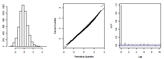
The key assumptions for NB models, and GLMs in general, are homogenous, Normal, and independent deviations centered on zero [65]. For our case, these assumptions are met and we present diagnostic plots for support (see Fig. (3)). From the histogram (left) and Normal quantile-quantile plot (center) of the model residuals, we have evidence that deviations are both Normal and centered at zero. From the autocorrelation plot of residuals, we find no evidence of dependence. Thus, our model form is valid.
7. VALIDATION
To validate our procedure and model specification, we perform a Cross-Validation (CV) procedure. Specifically, the CV technique used here is a repeated stratified random subsampling procedure where the data is tested against itself via training and testing subsets. Simple random sub-sampling to create training and test sets is not appropriate in our particular case since our model is estimating a random effect for route location. Thus, we need to ensure both training and testing sets contain the same routes, the random effect. This also means that some data are ‘lost’ since we have to omit data corresponding to routes with only one aggregate (only 7 routes had one aggregate). For each of the remaining routes (242), half of the associated aggregates were randomly assigned to a training set and the other half were assigned to a testing set (50% split).
Next, our NB model is fitted to the training set. The fitted regression parameters (based on the training set) and the observed values of the variables in the testing set are then used to predict the number of accidents in the testing set. This process was repeated 100 times, and for each repetition, for each route, 50% of the aggregates are randomly selected for training and testing sets.
To assess our model, we observe the root mean squared error, or RMSE, given by
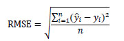 |
where
 is the predicted response (number of accidents), yi is the observed response (number of accidents), and n is the sample size. When we compare the RMSE from both the training and test sets, a good model will yield similar results. Otherwise, if the RMSE calculated from the training and test sets differ, we have evidence that our model is over-fitting or under-fitting the data. Since we produce an RMSE for the training and test set for each of the 100 iterations of our CV procedure, we have paired RMSEs and we used a paired test to identify potential differences. Assuming Normality in the differences, we have no evidence to suggest that the training and testing sets yield different RMSEs (t = 0.542, df = 99, p-value = 0.5887). We can conclude that our model is suitable and neither over- nor under-fitting the data.
8. DISCUSSION
We acknowledge that ‘human error’ plays an important role in roadway accidents [66, 67]. While we cannot detect this effect directly, we can quantify it indirectly. That is, we assume that human error will ‘emerge’ in the presence of certain roadway features, weather conditions, etc., and consequently, accidents will occur more frequently. Thus, we can consider our variables as catalysts, in some way, for human error.
In this work, we present a procedure aimed at identifying the relationships between roadway accident frequency and a variety of variables, and in so doing, we introduce several novel approaches. We present a segmentation/aggregation procedure that first breaks roadways into half-mile sections, then for accidents within each segment, a variety of roadway characteristics and features are identified. Next, we introduce a weather variable into our analysis by distinguishing accident totals by broad weather condition categories. Finally, we introduce a Negative Binomial (NB) regression model, a form that is theoretically justified, to identify the log-linear relationship between accident counts and roadway features, weather conditions, several interactions between weather and roadway features, and a random effect for the particular roadway.
Our procedure described above is applied to real-world data collected in Hamilton County, TN. Based on variation explained, model diagnostics, and a validation procedure, our methodology and model specification is justified. A novel result from our fitted model is the significance of several interactions between variables that are traditionally associated with accident frequency. Interpretations of coefficient estimates associated with these interactions are often logical or agree with current literature and the work of researchers in the field. Furthermore, statistically significant interactions suggest that the relationships between variables and accident frequency are nuanced, complicated, and cannot be described via main effects only. Understanding such relationships is critical to understanding the conditions associated with roadway accidents so that, ultimately, these conditions can be corrected [52].
Interpreting interaction terms from our fitted regression model, though sometimes complicated by categorical variables with several levels, leads to several interesting findings. First, when observing rural roads, cloudy conditions are associated with relative increases in accident frequency; and when observing the onset of rainy conditions, rural roads are associated with relative increases in accident frequency. Second, we find an interesting result related to the combined effect of AADT and continued, sustained rain. For low, average, and moderately high AADT, continued rain is associated with relative decreases in accident frequency; and for high AADT, continued rain is associated with relative increases in accident frequency. Third, considering the interaction between pavement width and AADT, we find higher AADT and wider pavements are associated with relative increases in accident frequency, whereas average AADT and wider pavements width are associated with relative decreases in accident frequency. Fourth, for higher speed limits, being in a residential area is associated with relative increases in accident frequency. These results illustrate the complicated relationship between accident frequency and both roadway features and weather. Furthermore, it is not sufficient to observe the effects of weather and roadway features independently as these variables interact with one another.
Like any work, there are a number of refinements that can be made to this work. First, our accident records have precise date and time designations, and it would be feasible to introduce a time-of-day, day-of-week, or season variable to our work. Related to this, Clarke et al. [68] showed how time-of-day (along with other variables) affects the crash frequency of young drivers, Qin et al. [69] revealed how the relationship between crashes and hourly traffic varies by time of day, and Laflamme and Ossebruggen [70] provided evidence of time-of-day and day-of-week effects on highway congestion which itself has been linked to accident occurrence [71]. We, however, opted for a more parsimonious approach, focusing on roadway characteristics and weather conditions. Second, our procedure does not consider the severity of accidents. Although severity information (such as fatality, etc.) was not available at the time of this analysis, including such information in the data aggregation procedure would be straight-forward. Numerous published works have performed analyses distinguishing between accidents of varying severity [12, 15]. Lastly, it has been shown that additional factors such as vehicle type [72, 73]; driver demographics such as age, gender, etc. [21, 74]; and driver state [75] play important roles in accident frequency/severity. Future work will pursue these variables.
CONCLUSION
Lastly, we acknowledge that our procedure makes several simplifications that could overlook important features. For example, among our weather variable categories, we do not distinguish between rain events of different intensity. Such data is available, and future work could introduce additional rain categories, or possibly create a continuous variable for the rain to account for varying intensity. Several works have investigated the effect of rain intensity on roadway accidents [23, 76].
CONSENT FOR PUBLICATION
Not applicable.
AVAILABILITY OF DATA AND MATERIALS
The authors confirm that the data supporting the findings of this research are available within the article.
FUNDING
None.
CONFLICT OF INTEREST
The author declares no conflict of interest, financial or otherwise.
ACKNOWLEDGEMENTS
The authors would like to thank the University of Tennessee at Chattanooga’s SimCenter. This work would not have been possible without their resources and support.

