All published articles of this journal are available on ScienceDirect.

The Effect of Ramp Proximity, Weather, and Time-of-Day on Freeway Accident Frequency: A Case Study on I-75 and I-24 in Hamilton County, TN
Abstract
Background:
We present a case study to quantify the dangers of freeway ramps by comparing the observed accident counts from ramp locations to those from adjacent mainline locations. Few works make this direct comparison. Additionally, time-of-day and weather information is considered to collect a deeper understanding of the nature of freeway accidents near ramps. Real-world data collected from freeways in Hamilton County, TN, are considered as an application and give interesting results.
Methods:
First, we precisely define ramp influence areas or areas within close proximity to ramp locations where traffic is suspected to be affected by the ramp structure/geometry. Then, we introduce a theoretically justified Negative Binomial regression model to approximate the relationship between accident counts (response), presence of ramp influence areas, and additional weather and time-of-day designations. Our model also considers selected interaction terms, route designation, and multiple random components that are aimed at explaining unmeasured sources of variation.
Results:
Based on the interpretation of our fitted statistical model, we find that being in an influence/ramp area (compared to being in mainline traffic), on average, results in a 4-fold increase in accident frequency. Moreover, we find that during clear conditions, rush hour conditions increase the accident frequency substantially, while during rainy conditions, this increase is much less stark. During non-rush hour conditions, rain decreases the accident frequency substantially, and during rush hours, this decrease is intensified. Model diagnostics and a validation procedure further justify the assumed model form and lend credence to our results.
Conclusion:
While we do not make any claim of transferability of our results, they provide a proof-of-concept that accident frequency is attributable to multiple factors, among which is proximity to ramps. Furthermore, our procedure and statistical model allow us to directly quantify how these factors, most notably ramp traffic, effect accident frequency. These results illuminate potential safety risks. Subsequent work considering more diverse roadways could provide the evidence needed for policy changes and/or remedial measures.
1. INTRODUCTION
Freeway off-ramps (exit ramps) and on-ramps (entrance ramps) are short sections of road that allow vehicles to, respectively, exit and enter a controlled-access highway. Locations near ramps often require sudden acceleration /deceleration as drivers respond to several complex events, such as merging, maneuvering, reading road signs, etc., all while trying to maintain a safe distance from other vehicles. Not surprisingly, this increase in volatility among drivers has been found to increase conflict and ultimately accident frequency [1]. As stated by Hu et al. [2], the complex interactions associated with merging, like those found at ramp locations, increased driver workload and the probability of errors. In fact, despite being relatively small portions of highway systems, locations near ramps are particularly dangerous and have been found to experience disproportionate numbers of accidents [3, 4]. According to the 2019 NHTSA report, there were more than 280,000 accidents on American highway ramps, almost 800 of which were fatal [5]. According to Torbic et al. [6], interchange-related crashes represent a substantial percentage of the safety concern on freeways.
Numerous works have investigated accidents at freeway ramp locations [3, 7, 10]. Some works have compared the effects of ramp type (on-/off-ramp, left/right exit) on observed accident counts [10], [7], but very few works have formally compared accidents at ramps to those occurring on mainline segments [8, 11, 12]. This is a primary goal of our work: to quantify the effect of ramp traffic on accidents. Furthermore, this work will consider additional sources, weather and time-of-day, to gain an insight into the general nature of accidents near freeway ramp locations – a holistic understanding of ramp accidents. Additionally, and not less importantly, we will introduce a rigorous statistical model that captures the true nature of accident data. To test the legitimacy of our approach, we will apply our procedure to real-world data from the two largest freeways in Hamilton County, TN, and our fitted model parameters will be interpreted to provide context.
We note that this work contributes to the field of traffic analysis in the following ways. First, it directly compares accidents at ramp locations with those occurring in adjacent mainline segments, an uncommon approach. This will allow us to directly quantify the ramp effect on accident counts. Second, additional sources of variability, weather and time-of-day, are considered. This results in a unique combination of explanatory variables that may allow us to identify complicated, nuanced relationships. Third, we introduce a theoretically justified count-based statistical model that will capture the variability of accident frequency and allow for physical interpretation.
We would be remiss not to note that ‘human error’ plays an important role, and likely a primary role, in roadway accidents [2, 13, 14]. While we cannot detect this human error directly (we do not have driver information prior to accidents), we can quantify it indirectly. That is, we can observe disruptions in traffic conditions that may force driver errors that can lead to crashes [15]. The explanatory variables chosen for this analysis are these disruptions, the conditions from which human error will emerge.
The remainder of this work is presented as a theoretically justified case study, with four broad sections. Section 2 (“Materials and methods”) presents several subsections which discuss the following: the presentation and justification of the statistical model to be used, the explanatory variables to be used with justification for their inclusion in the analysis, identification of influence areas to distinguish ramp and mainline traffic, the collection sites from which data are extracted, additional data sources, a data summary, our formal statistical model, and our model fitting procedure. Section 3 (“Results) presents a method for interpreting our fitting model results, the effect of our explanatory variables on the observed accident counts, model diagnostics, and a validation procedure. Section 4 (“Discussion”) gives perspective and interpretation of our findings/results, and section 5 (“Conclusion”) summarizes our work and identifies our important findings, some shortcomings or our procedure, and possible directions for future work.
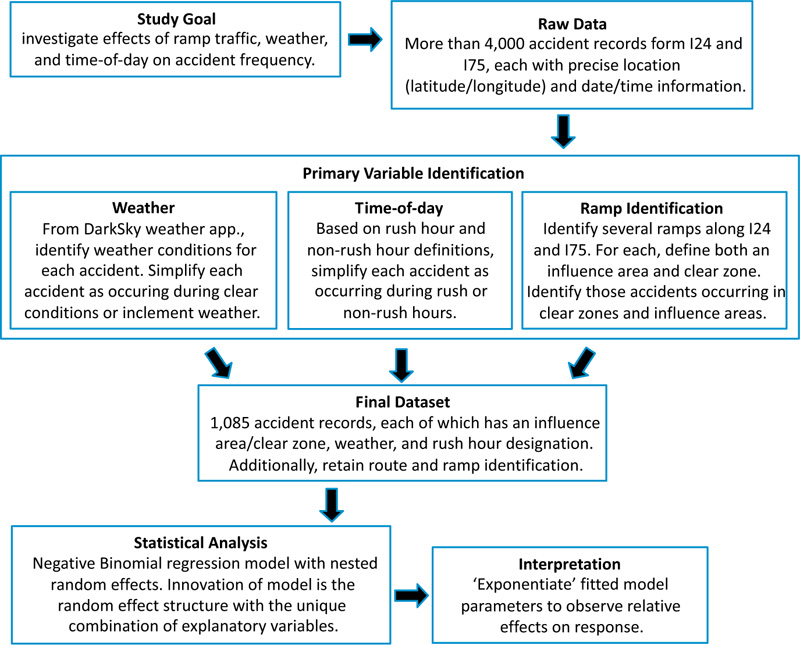
To assist the reader, the flowchart below Fig. (1) gives a concise summary of our experimental procedure.
2. MATERIALS AND METHODS
2.1. Mixed-effect Negative Binomial Regression Model
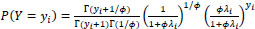
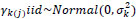
For our statistical modeling, we will ultimately use a Negative Binomial (NB) regression form. This first assumes that accident count data, Y, follows a NB distribution, or yi~NB(yi|λi, ϕ), with (eq. 1),
 |
(1) |
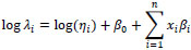
where λi >0 is the mean, ϕ is an over-dispersion parameter, and Γ(∙) is the Gamma function. The traditional NB regression model, then, has the following form (eq. 2):
 |
(2) |
where log (ηi) is an offset, β0 is an intercept, and βi are the model coefficients (to be estimated) associated with the predictors xi. This NB model form was pursued for two reasons. First, it is theoretically justified. There are several model forms that approximate count data such as traffic accidents. These include, but are not limited to, Poisson regression, Negative Binomial regression, and zero-inflated models. Since our final dataset contains very few zero values, the Poisson and NB forms were the logical forms to pursue. The Poisson form, however, assumes equi-dispersion, or the mean and variance of the data in question are the same (that is, E(yi) = Var (yi = λ), and this is not the case with our accident data. Thus, the NB regression model was pursued instead as this form includes a parameter to specifically account for over-dispersed data, the ϕ in (1). Thus, if
There is extensive literature supporting the use of the NB form for roadway accident counts, yet these works vary considerably in terms of scope. Chengye and Ranjitkar [8] used NB models and data collected from a highway in Auckland (NZ) to link accident frequency to ‘nonbehavioral’ factors such as traffic conditions, roadway characteristics, and weather conditions. Shankar et al. [16] used a NB model on data collected from rural highways to identify the relationships between accident frequency and roadway geometry, weather factors, and various interactions between them. Milton and Mannering [17] used the NB model and data collected from Washington highways to isolate the effects of geometric and traffic characteristics on annual accident frequency. Among other findings, the authors concluded that NB regression models are particularly appropriate for modeling accident counts, especially in instances where data are overdispersed relative to the mean. Abdel-Aty and Radwan [18] used the NB form to model the frequency of Florida highway accident occurrence based on roadway geometry, urban/rural designations, and section length. Other works using the NB model form for accident count data include Hauer et al. [19], Knuiman et al. [20], Miaou et al. [21], Hadi et al. [22], and Bauer and Harwood [7].
Because we will ultimately consider a selection of roadway locations (ramps from different routes) in our analysis, these locations will be used in our model as random intercepts (thus, we have a mixed-effects model containing both random and fixed effects). So, equation (2) becomes
 |
(3) |
where γj represents the random intercept for the jth location with γj~Normal (0,σ2). We assume that the different locations have differences/features that are site specific (roadway geometry, visibility issues, etc.). From the existing literature, it has been well established that such features are predictors of accidents in general [17] and specifically at ramp locations [7]. However, at the time of this analysis, we did not have a reliable way of identifying detailed roadway geometries for each location. Furthermore, some site-specific differences, such as human behavior, visibility issues, etc. are difficult or impossible to measure directly. The use of random effects overcomes this shortcoming in the data by allowing the counts to vary from location to location. In other words, random effects in our statistical model will allow for site-specific variation and essentially serve as catch-alls for sources of variation that are unobserved, unmeasurable, or simply too complicated to be modeled directly.
Several studies use NB model forms with random components. Gong et al. [23] applied a random-effect NB model to crash counts collected at different types of intersections. Wenfang et al. [24] found that a mixed-effects NB regression model was effective in predicting bus accident frequency on certain sections of roads in Nanjing, China. Chin and Quddus [25] used a random-effects NB model on data collected from signalized intersections in Singapore to identify relationships between accident occurrence and geometric, traffic, and control characteristics. Shankar et al. [26] explored NB and random-effect NB forms to approximate median crossover accident frequencies for several routes in Washington. Using roadway geometry, traffic volume, and a random effect to account for different routes, they found the random-effect model to be superior. In a related study, Ulfarsson and Shankar [27] compared NB and random-effects NB models to a Negative Multinomial model for accident frequency. Lastly, and germaine in this work, some studies have controlled for heterogeneity attributable to spatial and temporal correlation via random effects [28-30].
2.2. Ramps, Rain, and Rush Hour Traffic as Explanatory Variables
In our NB model, we consider fixed-effect explanatory variables related to ramp location, weather, and time-of-day. The goal of this study is to present a simplified procedure that gives a broad view of the nature of freeway accidents. In keeping with this goal, we identify the following simplified, dichotomous (binary) explanatory variables that distinguish 1) ramp area from mainline traffic, 2) inclement from clear weather, and 3) rush hours from non-rush hours. Such simplified variables also have the added benefit of making efficient use of what will ultimately be a limited dataset. That is, accidents are generally rare, and further focusing on ramp locations substantially reduces the available data. As suggested by Mannering and Bhat [31], simplified models may be necessary for situations where the data needed for more complex analyses are not available. We note that, in our statistical modeling, we also pursue the interactions between these simplified variables. In their analysis of safety performance functions, Islam et al. [32] identified the importance of incorporating interactions between variables for the estimation of accident prediction models.
Research suggests ramps are key features related to roadway accidents. In a work by McCartt et al. [3], Chi-square tests were used to significantly associate specific roadway/ramp characteristics with different types of crashes. Chengye and Ranjitkar [8] showed that, in addition to other roadway features, the presence of on- and/or off-ramps had a significant effect on accident counts. In comparing ramp and mainline segments, Van Beinum et al. [11] found that traffic is more turbulent around ramps due to route choice-related lane changes and anticipatory or cooperative maneuvers. Chen et al. [12] quantified the safety impacts of different types of exit ramps on freeway diverge areas. In their application of multiple correspondence analysis, Das et al. [33] found that on and off-ramps were associated with non-inclement weather crashes. Wang et al. [9] studied crashes on expressway ramps during periods of low visibility, finding an increase in crash likelihood as visibility decreases. Bauer and Harwood [7] used count-based regression models, both Poisson and Negative Binomial, to explore the relationships between traffic accidents and geometrics of interchange ramps and speed-change lanes. The authors collected accident data from both ramp and speed-change lanes and found that most of that variability in accidents was explained by ramp Annual Average Daily Traffic (AADT). Other works investigate ramps and specific types of accidents, such as those occurring in construction zones [34] or involving trucks only [35].
Next, weather conditions, especially precipitation/rain events, have been found to be important components of accident prediction [8, 9, 16, 36-41]. That said, the relationship between rain and accidents is not always straight-forward. Of course, positive relationships between rain and accidents have been established [39], but some works have found decreases in accidents with the onset of rain [8] or no significant association between rain and accidents [42]. The relationship between rain and accidents is likely complicated, nuanced, and depends on (interacts with) other factors. There are numerous studies illustrating the significant effect of weather interactions on roadway accidents. Laflamme et al. [43] found that the effects of weather are very much dependent on traffic volume and location. Shankar et al. [16] pursued numerous interactions between weather and geometric variables as part of their accident models. Wen et al. [44] found numerous interactions between weather conditions (wind, precipitation) and roadway geometry (curvature, slope) to be significantly correlated with freeway crash risk. Shankar et al. [45] found that weather, both as a main effect and interaction with roadside/traffic parameters, plays a statistically significant role in roadside crash occurrence. Jung et al. [46] found that a number of interactions with rainy conditions were positively associated with injury crashes.
Lastly, investigating the effect of rush hour on accident counts makes logical sense and allows for a sound statistical analysis of accident counts. As succinctly pointed out by Persaud and Dzbik [47], many statistical models tend to be macroscopic in nature as they relate accident occurrence to average daily traffic rather than to the specific flow at the time of accidents. As the authors point out, such models overlook rush periods when roadways have clearly different accident potentials. Using a dedicated rush-hour variable is an attempt to address and resolve this issue. Indeed, in their work in the application of generalized linear models to predict freeway accidents, Persaud and Dzbik [47] found that freeways associated with rush hour congestion were accompanied by greater collision risk. Other works have similarly used rush hour designations in their accident models. Using logistic regression models to predict the hourly likelihood of weather-related road accidents, Becker et al. [48] showed that, in general, probabilities had a pronounced diurnal cycle with maximum probability during morning and afternoon rush hours. Similar to our approach, Ma et al. [49] used a binary variable to distinguish between rush hours and non-rush hours in their logit model to predict the severity of auto crashes. In a study of time-series data mining models, Pan et al. [50] showed that considering rush hour behavior can improve the accuracy of predictors by up to 78%. Moreover, there are works that indirectly support the use of rush hour variables. It has been found that increased time pressure on drivers and traffic congestion is common during rush hours [49], and this combination of stress and congestion results in aggressive driving [51, 52], ‘turbulent’ traffic, and ultimately increases in accidents. Finally, it is worth mentioning that ‘rush hour,’ while primarily serving as a proxy for increases in volume, may serve as a ‘catch-all’ for other daily changes in traffic conditions. Such changes can include, but are not limited to, fluctuations in speed, increased aggressiveness, and even changes in light/glare.
In summary, as seen in section 2.1, several studies have shown the appropriateness of using the NB regression form to explain accident counts, and many of these models have used a type of random effect term. As seen above (in this subsection), numerous works have shown weather variables and time-of-day, especially rush hours, to be significant predictors of accident frequency. Moreover, as seen above, there have been studies that investigated the effect of different types of roadway features and ramps on accident frequency.
From our perspective, relative to the goals of this analysis, each work referenced has elements that can inform our own procedure, as well as elements that simply do not apply. That is, these referenced works are very much tailored to specific research goals or types of data, so no one approach can be used universally. Our goal, then, is to use the pros and cons of the existing literature to guide our own procedure. Many of the works referenced in section 2.1, particularly those using NB models with random effects, influenced our modeling approach, and these works lend credence to the appropriateness of such models. However, for our case, we need to extend these models to include nested random effects (to be discussed in section 2.7) to properly account for the nature of our particular data. To our knowledge, no published work has used a model such as ours. In this section (above), we discuss many works that investigated the association between accidents and some subset of ramp, weather, and time-of-day variables in their models. None, however, used this exact combination of variables, along with interactions between them. We pursued these variables (and interactions) because we consider them to be the primary, important, logical predictors of accidents, and we expect them to account for the majority of the variability observed in accident counts. In this way, we feel our results will fill a ‘gap’ in the literature by identifying a high-level, yet nuanced understanding of freeway accidents near ramps. Such understanding is necessary so that, ultimately, these conditions can be corrected or addressed [53].
2.3. Defining Influence Areas and Clear Zones
For this work, we need to devise a procedure for identifying freeway sections that can be used to address our research objectives. With a primary goal of investigating the relationship between accident frequency and proximity to on- and off-ramps, and to keep the analysis as simple as possible, we decided to discretize freeway sections near ramps into influence areas and clear zones. Very simply, influence areas are sections of freeway in close proximity to ramps where we expect to find a disproportionally high number of accidents. Clear zones, on the other hand, are areas set further away from the ramp, locations that are not expected to be directly and adversely affected by the ramp. We can think of clear zones as representative sections for mainline freeway traffic. The remainder of this section is devoted to defining influence areas/clear zones and justification for our definitions.
For off-ramp locations, the influence area is the section immediately before the exit, starting from the gore point and extending 1,500ft (457.2 meters) upstream. The corresponding clear zone is then the area starting at the upstream boundary of the influence area and extending an additional 1,500ft upstream. For on-ramp locations, on the other hand, the influence area is the section immediately following the entrance, starting from the gore point and extending 1,500ft downstream. The corresponding clear zone, in this case, is then the area starting at the influence area boundary and extending an additional 1,500ft downstream. See Fig. (2) below for an illustration of influence areas and clear zones.
If the length of a designated influence area is too long, the reported accidents may include mainline accidents or accidents not directly influenced by ramps. If the selected length is too short, however, we may not be able to assess the true influence of the ramp on freeway traffic. The lengths of our influence areas were chosen primarily based on the merge/diverge influence areas defined by the Highway Capacity Manual [54], which defines these areas as 1,500ft before and after off- and on-ramps, respectively. Similarly, a thorough work by Chen [55] defined influence areas of 1,500ft from gore points. Other works used influence areas between 1,000ft and 2,000ft from gore points [56-58]. Slightly longer and shorter influence areas were investigated with only subtle changes in the results. Regarding the use of fixed-lengths for traffic studies, Cafiso et al. [59] found that fixed-length segmentation (such as we have) is a flexible and statistically consistent technique, and other works have used fixed-length segments to study traffic accidents [43, 60].
Next, while there may be some merit to defining ramp locations to include areas downstream of off-ramps and upstream of on-ramps, we decided against this to focus solely on the areas similar to the merge/diverge influence areas defined by the Highway Capacity Manual [54]. Prior investigations of the data suggest that areas upstream of off-ramp and downstream of on-ramp are the most important locations in terms of accident occurrence. Research supports this. In a thorough work by Hossain and Muromachi [15], a random multinomial logit model was used to identify significant predictors of accidents near ramps on a Tokyo expressway. The authors found that only the locations upstream of an off-ramp and downstream of an on-ramp (our influence areas, as defined) were useful predictors. They concluded that maneuvering mainly occurs downstream of on-ramps and upstream of off-ramp, and these areas have more detectable interruptions in the mainline traffic flow. Finally, and importantly, extending the influence downstream of off-ramp location and upstream of on-ramp location could likely introduce areas with dissimilar crash features and influential factors.
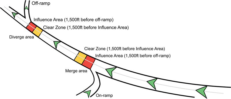
As previously mentioned, each influence area has a corresponding clear zone of the same length of 1,500ft. This was done intentionally to make the clear zones and influence areas more comparable and limit any potential change in exposure. That is, if the corresponding clear zones and influence areas are of the same length (and have the same collection period as they do), we do not have to specifically account for such differences in our statistical modeling and we can, potentially, more easily identify the true sources of accident variables between the areas. Moreover, these clear zones represent mainline traffic that is NOT influenced by the presence of an off- or on-ramp, and Chen [55] found, from field observations, that ramps had little influence on mainline traffic beyond a length of 1,500ft. We acknowledge that this is a general approach and that the dimension of an influence area is likely dictated by numerous factors such as ramp type (entrance or exit), speed limit, ramp curvature, visibility, and other features. In other words, the unique features of the ramp determine the exact dimensions of the influence areas. Because much of this information was not available, and to keep the procedure as simple as possible, we opted to use a constant influence area length for all locations. Lastly, we note that the ramp locations chosen for this analysis are somewhat similar (comparable speed limits, no overlapping influence areas, no ‘complicated’ ramp structures, etc.), and our influence area is believed to work, in general, for these cases.
2.4. Collection Sites
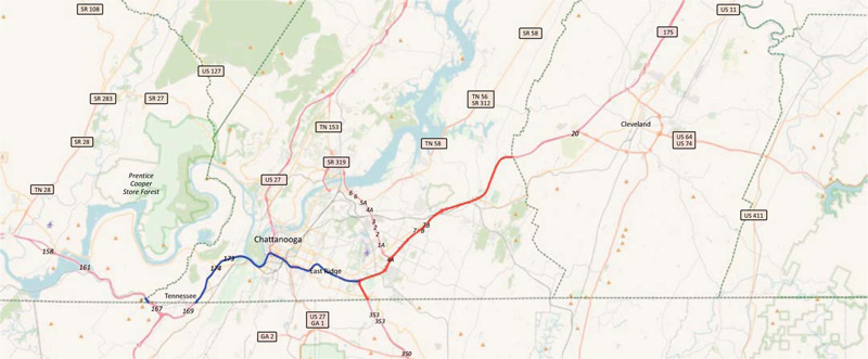
As mentioned throughout this work, freeway ramps are the focus of this analysis, and as such, the two major interstate highway systems in Hamilton County, Interstate routes I75 and I24, were used as collection sites. Both I75 and I24 are interstate freeways/highways with between 2 and 6 lanes of one-directional travel. Route I75 starts at the GA state line in the south/central portion of Hamilton County and travels in the northeast direction for approximately 15.6 miles (see Fig. (3) below, red line). Route I24 begins in the southwest portion of the county at the GA state line and runs in the east/west direction for approximately 14.7 miles until it connects with I75 (see Fig. (3), blue line). These routes are ideal collection sites as they both contain numerous on- and off-ramps, observe frequent roadway accidents, and experience heavy daily traffic with AADTs exceeding 120,000 at some locations. Both I75 and I24 have north/south and east/west directional distinctions, respectively, and we suspect there may be some differences between them. For our statistical model, the ‘route’ variable will distinguish between the four categories: I75North, I75South, I24East, and I24West.
2.5. Merging Datasets
A major task associated with this work is the creation of a dataset amenable to the envisioned procedure. To do this, we will need to identify all accidents occurring in the influence areas and clear zones along I75 and I24 (as defined above), and then further specify these accidents by time-of-day and weather conditions. To do this, we require three sources of data: Hamilton County emergency services, the DarkSky weather application, and the Tennessee Department of Transportation (TDOT) enhanced Tennessee Roadway Information Management System (eTRIMS) database (https://e-trims. tdot.tn.gov/etrimsol/web/).
First, based on dispatch information collected from first responders (police, fire, and EMS), the Hamilton County Emergency Communications Center provided information for all traffic accidents along I75 and I24. At the time of data acquisition, accident information was available between January 1, 2017 and December 31, 2018, a 2-year collection period. Importantly, each accident record has an associated physical location in terms of route, latitude/longitude, and mile marker designations.
Next, using TDOT’s eTRIMS (https://e-trims.tdot.tn.gov) referencing database for roadway structures, we were able to precisely identify the gore point location of on- and off-ramps along I75 and I24. Then, the influence area and clear zone boundaries are defined by identifying two successive 1,500ft sections upstream/downstream of off-/on-ramp locations. At this point, we can easily identify every influence area and clear zone in terms of mile marker and route. Each influence area and clear zone was then assigned an accident count by matching accidents to the boundaries of these areas.
As a penultimate step, weather conditions were incorporated into the dataset. Based on physical location and time/date information (both provided by Hamilton County Emergency services), we were able to link each accident to specific weather conditions. These conditions were identified by using the DarkSky weather application (https://darksky.net), an API for Python that collects weather data from several weather resources and makes available information associated with specified locations at precise time periods. To simplify the process, clear and cloudy conditions are combined into one classification called ‘clear;’ and rainy, foggy, and snowy conditions are combined into one classification called ‘rainy.’ We then introduce a categorical variable to distinguish between the two classifications: clear (actually clear or cloudy) and rainy conditions (actually rainy, foggy, or snowy). While different studies used varying degrees of simplification, it is not uncommon for researchers to discretized categories of weather conditions when studying the effects of weather on accident risk [36].
Lastly, based on time records collected by the Hamilton County emergency services, each accident was identified as either a “rush hour” accident or “non-rush hour” accident. As is somewhat standard, the rush hour was identified as between 6-9AM and 4-7PM. While this may seem like a coarse simplification, distinguishing between these periods is perfectly sufficient to provide interesting, meaningful results that would be of general interest to city planners, freeway administrators, etc.
Based on previous work [61, 62], we suspect that weekend traffic does not follow the same rush hour trends observed during the week. Furthermore, it is likely that recreational, weekend travel has a higher potential for accidents. Because of these potential differences, considering weekend accidents in our analysis would surely require an additional variable to distinguish weekend from weekday accidents. In our opinion, this would make for an overly complicated model. For simplicity, and to maintain homogeneity in the dataset, we decided to focus exclusively on weekday (Monday-Friday) accidents. In an analysis to identify accident hotspots and improve prediction methods, Amili [63] found that weekday and weekend traffic volumes (collected from expressways in central Florida) differed substantially and demanded separate analyses.
2.6. Data Summary
Along I75, twenty (20) ramps were selected: 9 from I75North, 11 from I75South. These ramps are situated at highway locations with between 2 and 4 lanes of travel, and posted speed limits at these locations vary between 55 and 65 mph (between 88.5 and 104.6 kph). During the collection period, near these ramps, there were a total of 516 accidents observed (204 for I75North, 312 for I75South), or about 24% of all accidents occurring along I75. Along I24, eighteen (18) ramps were selected: 9 from I24East, 9 from I24West. Like the locations along I75, these ramps are situated at locations with between 2 and 4 lanes of travel, and posted speed limits at these locations vary between 55 and 65 mph. During the collection period, near these ramps, there were a total of 569 accidents observed (409 for I24East, 160 for I24West), or about 28% of all accidents occurring on the route.
Among the 38 total freeway ramps on the four routes, 1,085 total accidents were considered for this analysis. For each of these accident records, we have the ramp/route, section type (influence area or clear zone), weather (clear or rainy), and rush hour (rush hour or non-rush hour) designations. These designations are the categorical explanatory variables to be used in this analysis. Table 1 (below) gives the distribution of the 1,085 accidents across all categories of explanatory variables.
| Categorical Variable | Category | No. of Accidents | Proportion of Total Accidents |
|---|---|---|---|
| Route | I-75 North | 204 | 19% |
| I-75 South | 312 | 29% | |
| I-24 East | 409 | 37% | |
| I-24 West | 160 | 15% | |
| Section type | Influence area | 878 | 81% |
| Clear zone | 207 | 19% | |
| Time-of-day | Rush hours | 698 | 64% |
| Non-rush hours | 387 | 36% | |
| Weather | Clear or cloudy | 930 | 86% |
| Rain, fog, or snow | 155 | 14% |
Not every ramp along I75 and I24 was considered for this analysis. There were several ‘ramp systems’ that contained two or more ramps that were very close together. Such combinations of ramps were deemed unusable because their influence areas/clear zones, as we have defined them (1,500 feet before/after gore point), overlapped with other influence areas/clear zones. In these cases, accidents could occur simultaneously in influence areas and clear zones, so these confounding cases were disregarded. Furthermore, any accidents occurring at these locations are potentially caused by a flawed design and not simply the influence of the ramp. We feel justified, then, not to consider such locations in our analysis. The 38 ramps used in this analysis were ‘simple’ cases that had no interference with other ramps or roadway structures (locations in which the ‘ramp effect’ could be isolated).
The 38 influence areas (one per ramp) had an average of 23.11 accidents and a standard deviation of 21.53, whereas the 38 corresponding clear zones had an average of 5.45 accidents and a standard deviation of 5.5. So, as compared to the clear zones, the influence areas have a higher average and higher variability in accident counts.
2.7. Statistical Modeling
A Negative Binomial regression model was ultimately selected for our analysis as our data exhibits over-dispersion. As stated, the Negative Binomial model form, compared to the simpler Poisson form, includes an additional parameter to account for this over-dispersion, and thus it is a more flexible model. We note that more exotic versions of Negative Binomial models were also pursued, namely zero-inflated and hurdle variants. However, based on likelihood ratio tests and comparison of AIC scores, these more complicated models were not preferred. Formally, our Negative Binomial mixed-effects regression model is
 |
(4) |
where λijk is the mean accident count at the ith observation (i = 1,…,6), jth ramp (j=1,…,nk), and kth freeway route (k=1,…,4); ϕ is the Negative Binomial over-dispersion parameter with the variance of counts given by
 and Ɛk(j), γk(j) are nested random effects. The nested random effects, then, require a more complicated NB regression form than equation (3). Specifically, we have,
 |
(5) |
 |
(6) |
 |
(7) |
where log (ηijk) in is an offset; β 0 is an intercept; xdijk is a set of indicator variables for  (equations 5 and 6) to account for variation by ramp within route; and Ɛk(j) is a nested random effect with associated ΣAR (1) autoregressive covariance matrix (equation (7)) to account for the serial correlation related to the position of the ramp within route. Since the ramp locations used in this analysis represent a selection of all such locations along the two routes, they are theoretically justified as random effects.
Very often, count-based regression models like the Negative Binomial include an ‘offset variable’ to account for disparate ‘exposures’ in the data. In our case, all influence areas and clear zones are equally spaced (1,500ft length), and the collection period is constant (2 years), so our primary source of variation in exposure comes from changes in volume between freeway locations. High traffic flow (represented by AADT, hourly volume, etc.) is generally considered to increase the risk of crashes on roadways [17, 18, 64] and specifically on freeway ramps [7, 56]. For this reason, and based on numerous other works that have used AADT as an offset in count-based models (for example), AADT will be set as an exposure/offset variable (in our model above, ηijk represents the AADT of observation ijk). Importantly, although this structure assumes a linear relationship between AADT and traffic counts, our time-of-day variable accounts for intraday changes in traffic behavior (flows) that occur daily. Thus, these model components, when considered together, address the potential nonlinear effect of traffic flow on accident counts.
Based on the current literature, some works have used similar models (NB regression with random effects), and other works have used some combinations/subsets of variables in this analysis (weather, time-of-day, etc.). However, no work, to our knowledge, uses this type of model with a nested random effect structure and a variable to distinguish ramp traffic from adjacent mainline traffic. These novel elements are logically/theoretically justified, but subsequent sections will provide further support for our model.
2.8. Model Fitting
All data manipulation and statistical analyses were performed using the R statistical software system [65] and its base packages. Additionally, model fitting of the generalized mixed models was performed using the ‘glmmTMB’ package [66] via maximum likelihood estimation and 'TMB' (Template Model Builder).
As a first analysis of the model-fitting results, we checked if the NB model form itself is justified. That is, is the data sufficiently over-dispersed to warrant the NB model form which contains an additional parameter to account for this extra spread? Or, if the data is not over-dispersed, will a Poisson form suffice? Since the Poisson model form is nested within the NB model form (the NB model has one additional parameter to account for the over-dispersion), we performed a likelihood ratio test to assess whether or not the use of the more complicated model, the NB model, is necessary. In our case, the dispersion parameter, ϕ, was found to be 4.33, and as suspected, the NB model form was a statistically significant improvement over the simpler Poisson model (Likelihood ratio X2 = 29.235, df = 1, p-value < 0.0001). Moreover, numerous versions of more exotic models (for example, NB, hurdle, and NB with zero inflation) were tested and none provided a significantly better fit to the data. Thus, the ‘standard’ NB model form was justified.
Related to the random effects in our mixed model, a complication arises in the testing of such effects. That is, to test these effects, we are essentially testing whether or not the variance parameter is zero. Since the variances must be zero or positive, a test of zero is on the border of the parameter space, and the tests of parameters are valid only on the interior of their space. Thus, direct tests are not recommended or justified. Moreover, and importantly, we feel the random components reflect an important, fundamental structure in the data. They represent sources of variability in the data not accounted for by our other explanatory variables. Thus, they will be estimated and retained without direct testing.
3. RESULTS
3.1. Preliminary Comments
Since we assume an NB form, our explanatory variables have a log-linear relationship with our response variables, so the estimated parameter values must be ‘exponentiated’ to assess their relative effect on the response variable (that is, we need to calculate an ‘incidence rate ratio’). The NB regression form
 |
may be expressed as
 |
 |
(8) |
As we can see from equation (8), for some fitted coefficient βp, exp {βp} gives the multiplicative effect on the mean response for each unit increase in xp. Conveniently, our fixed effects are dichotomous (xp take values of 0 or 1 only) so that the exp {βp}. quantities are interpreted as relative effects on the response when the qualitative attribute is present (versus the base case). Lastly, for mixed models, such as we have here, statistical tests of fixed effects are typically based on either Wald or likelihood ratio (LRT) tests (the two are equivalent, given a suitable sample size). Using the ‘car’ package [67] in R, we produced Wald tests for our parameter estimates, which test effect sizes scaled by the estimated standard error. After a stepwise removal of insignificant terms, a final model was identified and Table 2 below gives the Wald test results for selected significant variables.


Second, we address the overall effectiveness of our model to explain the observed variability in the accident counts. For a mixed-effects model, an R2 value is not readily available from the model output. Instead, we can calculate an R2 substitute/alternative from the residual variances. Specifically, we use the following.
 |
(9) |
where Vnull is the variance of the residuals from the null model (the model with only an intercept and random effects) and Vmodel is the variance of the residuals from the full model. This R2 from equation (9) can be interpreted as the additional variance explained by the fixed effects over that explained by the random effects. In our case, we find R2 = 0.79. This means that the explanatory variables (those listed above in Table 2), even though they are discretized/simplified, explain a high majority of the variance observed in the accident counts. This result gives credence to our procedure and the selection of variables.
3.2. Influence Area
Since we consider just the two categories of influence area and clear zone, the corresponding variable representing the influence area is binary and takes values of 0 and 1 when our freeway segment is in the clear zone (or not in the influence area) and when our segment is in an influence area, respectively. That is, the clear zone is essentially the baseline category and the influence area is the adjustment to it. Using the property put forth in equation (8), we find that the influence area affects the number of freeway accidents by a factor of exp{1.471(1)} = 4.355, or is associated with more than 4-fold increase in accident frequency compared to being in the clear zone (base case, when the binary variable is set to 0) or a segment more representative to mainline traffic. We note that interpreting and generalizing our results should be done cautiously. Our fitted parameter estimate is likely specific to the source of the data, the 38 ramp locations along I75 and I24 in Hamilton County (TN), and only provides evidence that accident frequency significantly increases in influence areas.
Most ramp studies focus exclusively on accidents occurring within ramp locations [7], and do not compare accident counts between ramp and mainline freeway segments (as we have done). Thus, direct comparison of the results to the existing literature is difficult. In an early work studying freeway exit ramps, however, Taylor and McGee [68] reported that erratic maneuvers are a common occurrence at these locations, and that the number of crashes there is four times greater than at any other freeway location (a result similar to our results above).
Lastly, we note that several interactions involving ‘influence area’ were pursued (influence area by weather, influence area by rush hour, etc.), yet none were found to be statistically significant predictors. This is itself interesting in that it suggests the effect of the influence area on the accident count is, for the most part, constant across different levels of the other variables. Again, we interpret this result with caution and note that both weather and rush hour variables were both highly simplified into two categories. Using more nuanced categories may result in the identification of significant interactions. For example, observing rain across a continuum of intensities may help to identify some significant (and interesting) interactions with the influence areas. Along these lines, Malin et al. [36] investigated numerous types/intensities of precipitation on different types of roadways. The authors found that the effect of different precipitation on roadway risk varied by the type of roadway.
3.3. Rush Hour and Rainy Weather
Because rush hour and rain have a significant interactive effect (see Table 2 above), their effects on accident counts cannot be identified independently. That is, the significant interaction between rush hour and rain means that the effect of rain on the accident count depends on the level of rush hour, or equivalently (from the other perspective), the effect of rush hour on the accident count depends on the level of rain. Moreover, since neither rush hour nor rain interacts with the influence area (see above), our interpretation of rush hour and rain applies to both the influence area and clear zone accidents.
From the rush hour perspective, when the rain variable takes a value of 0, or when we have clear/cloudy conditions (no rain), rush hour affects the number of freeway accidents by a factor of exp{0.743(1) − 0.558(0 * 1)} = 2.102, or is associated with about a 2-fold or 110% increase in accident frequency compared to being in non-rush hour conditions (base case, when the rush hour variable is set to 0). However, when the rain variable takes a value of 1, or when we have rainy weather conditions (actually rain, fog, or snow, but simplified as ‘rainy’ conditions), the rush hour affects the number of freeway accidents by a factor of exp{0.743(1) − 0.558(1 * 1)} =1.20, or is associated with just a modest 20% increase in accident frequency compared to, again, being in non-rush hour conditions. This is the interaction effect: rush hour conditions affect the accident frequency, but the precise effect depends on the weather. More summarize more specifically, if it is clear (no rain, fog, or snow), rush hours increase the accident frequency substantially by about 110%; if it is rainy (rain, fog, snow), rush hours increase the accident frequency more modestly, by about 20%.
Can we explain this result? It is difficult to find direct support for this result in the existing literature as few studies have looked at the interaction of rush hours and rain events. Certainly, our results during clear conditions make sense as several works have verified that accidents increase during periods of increased volume/rush hours [47, 48]. However, during rainy conditions, we observe a more modest increase in accident frequency. Why is this? A possible explanation is that inclement weather may reduce traffic volumes and aggressive driving (because of decreased visibility, increased driver caution, etc.) typically seen during rush hours. Therefore, instead of compounding the effect with increased volume/congestion, the rain lessens the effect. At the very least, this result illustrates the very complicated, nuanced relationship between driving conditions and accidents. We can try to explain our findings mechanistically by looking at the observable effects of rain on traffic. Research has shown that adverse weather can result in decreases in traffic volume [69], decreases in speed [70], and increases in mean headway [71]. It is possible, then, that slower speeds and increased spacing reduce the dangerous effects of rush hour conditions.
Next, from the rain perspective, when the rush hour variable takes a value of 0, or when we observe off-peak hours (non-rush hour), the rainy weather affects the number of freeway accidents by a factor of exp{−1.456(1) − 0.558(0*1)} = 0.233, or is associated with a 76% decrease in accident frequency compared to being in clear conditions (base case, when the rainy variable is set to 0). However, when the rush hour variable takes a value of 1, or when we observe peak traffic conditions, the rainy weather affects the number of freeway accidents by a factor of exp{−1.456(1) − 0.558(1*1)} = 0.133, or is associated with an 87% decrease in accident frequency compared to, again, being in clear conditions, but simply from the point of view of weather. To summarize, during non-rush hour conditions, rain decreases the accident frequency substantially, and during rush hours, this decrease is intensified.
Can we explain this result? At first glance, the results above may seem surprising (that rain generally decreases the frequency of accidents) since many studies suggest roadways generally become more dangerous during rain and inclement conditions [36]. However, we only consider highways/freeways in this analysis, and some studies, particularly those focusing on similar roadway types, support our result. A multi-year study by Peltola [72] found that a majority of traffic accidents on “main roads” occurred during clear/cloudy weather conditions (incidentally, the same distinction was used in this study). Also, Chengye and Ranjitkar [8] found a decrease in city highway accidents with the onset of rainy weather, likely attributable to the fact that traffic volume is reduced on rainy days, and drivers are more cautious. Moreover, Eisenberg [39] generally (for all roadway types) found a negative correlation between monthly precipitation and fatal accidents. As stated by Edwards [73], “…relationship between adverse weather and road accidents is far from straight-forward.”
3.4. Model Diagnostics
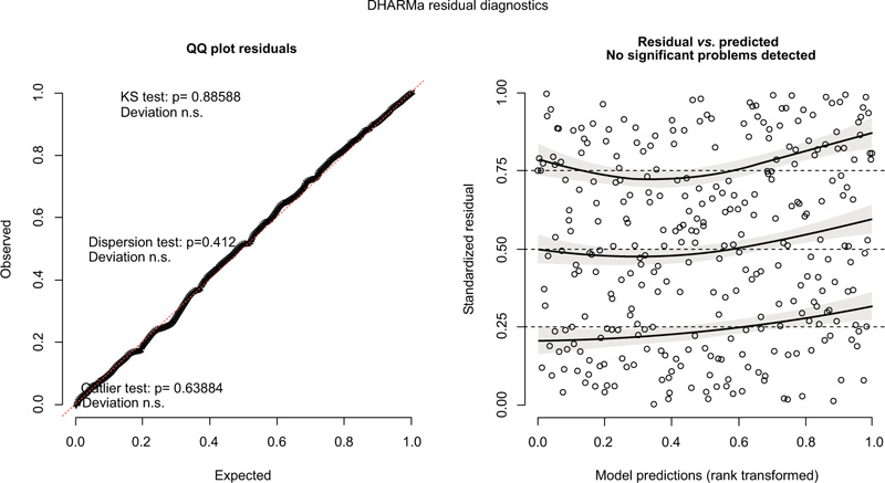
A well-known issue with generalized linear mixed models is that it is difficult to diagnose misspecification problems with the assumed model form. Specifically, there are few checks for the entire model structure, including all levels of random effects. To address this drawback of generalized linear mixed models, the ‘DHARMa’ package for R [74] was created to assess the appropriateness of model specifications. The DHARMa package uses a simulation-based approach to create interpretable, standardized residuals (with values between 0 and 1). Essentially, the observations are compared to the empirical cumulative density functions associated with each predicted value. Fig. (4) presents the DHARMa diagnostic plots associated with our model.
On the left plot, we have a quantile-quantile plot to detect overall deviations from the expected distribution with added tests for the correct distribution (Kolmogorov-Smirnov Test), dispersion, and outliers. Here, adherence to the transverse line suggests that our model form is appropriate. For the K-S test, we have a p-value (for K-S test) of 0.88, and NO evidence that our model is incorrectly specified. On the right, we have a plot of the standardized residuals against the predicted values with additional empirical 0.25, 0.5, and 0.75 quantiles (solid black lines) from theoretical 0.25, 0.5 and 0.75 quantiles (dashed black lines) to help detect deviations from uniformity. Here, the residuals look uniform (no curvature, change in variance), and the test of deviation of these residuals from their quantiles has an associated p-value of 0.29. Thus, again, we have no evidence of incorrect specification. We can conclude that our model, as specified by the variables chosen, accurately approximates the data and can explain the observed accident counts without overlooking some major underlying trend. In an application by Zhang [75], a Poisson model with spatially dependent random effects was used to approximate the accident counts of teenage drivers. As above, the authors used the DHARMa package and the resultant QQ plots of the residuals to conclude that their model was correctly specified.
3.5. Model Validation
To validate our procedure and model specification, we perform a cross-validation (CV) procedure. The CV technique used here is actually a repeated, stratified random subsampling procedure with training and testing subsets of the data. Such a procedure is necessary since our model estimates two random components nested in the four route locations. For each ramp, two of the eight counts were randomly assigned to a testing set and the remaining six counts were assigned to a training set (so, 75%-25% training-testing split).
Next, our mixed-effects NB model was fit to the training set. The fitted regression parameters (based on the training set) and the observed values of the variables in the testing set were then used to predict the number of accidents in the testing set. This process was repeated 100 times with training and testing sets randomly chosen in each iteration. As a first assessment, we use the root mean square error (RMSE) to determine if the model is under- or over-fitting the data. The RMSE is given by
 |
(10) |
where y^i is the predicted number of accidents, yi is the observed count, and
Lastly, to assess the predictive ability of our model, we employ a multiclass ROC analysis. The area under the ROC curve (AUC) is a widely used measure of the performance of supervised classification rules. The traditional ROC is applicable to the two-class case but has been extended to the case of more than two classes [76]. This multiclass ROC averages pairwise comparisons between classes and the resulting AUC calculation has essentially the same interpretation as that of the two-class case. For each of the 100 iterations of training/testing described above, we calculated the multiclass AUC via the ‘pROC’ package in R [77]. From these 100 AUCs, the resulting 95% confidence interval for the test set is (0.837, 0.914). Interpreting AUC is subjective and relative, but this result indicates that our model (as specified) is, by most standards, a very good predictor of accidents.
4. DISCUSSION
Related to our procedure, there are numerous refinements that can be made. There is some evidence that more accidents are observed near off-ramps than on-ramps [7] and different ramp types have different effects on accident frequency [78] and [10]. Although not discussed previously, a separate analysis of the same data failed to find significant differences between on- and off-ramps, but no distinction between ramp types was pursued. At the time of writing, detailed descriptions of ramps were not available, but future work could distinguish between broad categories of ramps. Furthermore, location-specific details (road geometry, visibility, speed limits, etc.) surely play an important part in defining influence areas. Future work will pursue defining influence areas precisely based on roadway features near ramps. Next, as discussed previously, we only consider weekday/commuter accidents in this analysis. Weekend/recreational travel may likely contribute to accident occurrence, and future analyses will pursue these cases. Next, our procedure does not consider the severity of accidents. Although severity information (such as fatalities, etc.) was not available at the time of this analysis, including such information in the data aggregation procedure would be straightforward. Numerous published works have performed analyses distinguishing between accidents of varying severity [79]. Next, it has been shown that additional factors such as vehicle type [80] driver demographics such as age, gender, etc. [18] and driver states [81] play important roles in accident frequency/severity. Future work will pursue these variables. Lastly, we acknowledge that our procedure makes several simplifications that could overlook important features. For example, among our weather variable categories, we do not distinguish between rain events of different intensities. Such data is available, and future work could introduce additional rain categories, or possibly create a continuous variable for rain to account for varying intensity. Several works have investigated the effect of rain intensity on roadway accidents [82].
In their review of current accident analysis techniques, Gutierrez-Osorio and Pedraza [83] state, “the study of road accident prediction is…open to innovation in the research of algorithms and data analysis techniques…” Future work in the area will likely pursue such modern analysis techniques to more accurately model accident counts and/or identify factors associated with accident occurrence. There are numerous works investigating the effectiveness of these innovative techniques on accident data. Ren et al. [84] used a type of deep learning model, called a long short-term memory (LSTM) architecture model, to predict traffic accident risk. Based on spatial and temporal traffic accident data collected from Beijing, their model outperformed other, more traditional models. Ait-Mlouk and Agouti [85] used association rule mining, a technique that extracts correlations among different attributes in a dataset, to analyze road accidents in Morocco. The authors were able to identify meaningful relationships between certain variables and roadway accidents. Moriya et al. [86] explored the use of a clustering algorithm (using Bayesian information criterion (BIC) and Akaike information criterion (AIC) for cluster selection) to predict accident counts and to identify risk factors. Using traffic date from Tokyo roads and intersections, the authors successfully identified three distinct clusters of locations based on riskiness. Generally, these modern techniques ably address complicated combinations of variables, and we are optimistic that future work using such techniques will discover interesting relationships.
CONCLUSION
In this work, we present a procedure aimed at identifying the relationships between roadway accidents and explanatory variables based on proximity to ramp, weather, and time-of-day conditions. Among these, the variable identifying ramp traffic is of primary importance as it will potentially allow us to quantify the effect of ramps on accident frequency, a topic that has received little attention to date. To test the legitimacy of our procedure, we apply our methodology to real-world accident data from Hamilton County, TN.
Our work requires substantial preprocessing to create a dataset amenable to our analysis. That is, we have to ‘build’ a dataset of accident counts and associated ramp designations, weather conditions, and time-of-day. To do this, we first develop a method of distinguishing ramp traffic from adjacent mainline traffic. We define the short sections immediately upstream/downstream of exit-/on-ramps, respectively, as influence areas or areas potentially affected by ramp traffic. The sections further upstream/downstream of these segments are considered clear zones, or areas representative of mainline traffic. Along our freeway collection site, 38 suitable ramps are chosen, and influence areas and clear zones are identified for each. Then, from Hamilton County emergency services records, accident counts are assigned to each influence area and clear zone. Finally, time-of-day information and weather conditions are assigned to each accident from accident reports and the DarkSky weather application, respectively. This time-of-day and weather information is ultimately simplified to distinguish between rush/non-rush hours and clear/rainy conditions, respectively. In the end, our dataset contains 1,085 accident records, each of which has an associated ramp/route, rush hour, weather (clear or rainy), and section type (influence area or clear zone) designation.
A statistical model, a Negative Binomial (NB) regression model with both fixed and random effects, is pursued to provide the link between accident counts and our explanatory variables. A benefit of the regression form is the interpretability of the fitted model parameters. That is, the fitted parameters will allow us to quantify the relative effect of variables on the response. A novel aspect of our procedure is the inclusion of several interactions between variables that are traditionally associated with accident frequency. The model is applied to our dataset, and based on the model diagnostics and a validation procedure, our methodology is justified. This type of model, with this combination of explanatory variables, appropriately captures the majority of the variability (more than 79%) observed in accident counts.
Interpreting the fitted regression parameters leads to several interesting findings, many of which are logical or agree with the current literature and the work of researchers in the field. First, compared to being in the clear zone (or mainline segment), being in an influence area, on average, results in about a 4-fold increase in accident frequency. In addition to this, and interestingly, the influence area was not found to interact with any other variables, so the effect of the influence area on the accident count is roughly constant across these other variables. While it may seem intuitive, this result is the major finding of this work. We are able to directly compare ramp locations to adjacent mainline segments and ultimately quantify the effect of ramp traffic.
An interesting result from the fitted model is the statistically significant interaction between rush hour and rain variables. This tells us that the two variables are dependent and that their relationship with accident frequency cannot be described via main effects only. Interpreting our fitted model parameters, we find that during clear conditions, rush hour conditions increase the accident frequency substantially, while during rainy conditions, this increase is much less stark. Or, we can interpret this interaction from the other point of view, in terms of weather. During non-rush hour conditions, rain decreases the accident frequency substantially; and during rush hours, this decrease is intensified. These interpretations illustrate the complicated relationship between rush hour conditions and inclement weather, and how their relationship with accident frequency is nuanced.
Clearly, because this is a case study with just two freeways, we cannot make any recommendations to administrators based on our findings, nor do we claim that our results are transferable to freeways in general. However, we believe our work has identified some interesting relationships and stands as a proof-of-concept. Subsequent work considering more diverse roadways and/or ramp locations could provide more general results and potentially the evidence needed for policy changes and/or remedial measures. Such measures include structural changes such as widening, striping, and canalization, but may also include ramp metering which would regulate traffic flow and mitigate collisions, particularly those during rush hours. Currently, there is a rich field of sophisticated, state-of-the-art methods to optimize flow through complicated systems [87], some of which have clear application to freeway ramps.
CONSENT FOR PUBLICATION
Not applicable.
AVAILABILITY OF DATA AND MATERIALS
None.
FUNDING
None.
CONFLICT OF INTEREST
The authors declare no conflict of interest, financial or otherwise.
ACKNOWLEDGEMENTS
This analysis would not have been possible without the cooperation of the Center for Urban Informatics and Progress (CUIP) at the University of Tennessee at Chattanooga and its director, Dr. Mina Sartipi. The resources and relationships made available to us through the CUIP were invaluable to our work.

