All published articles of this journal are available on ScienceDirect.

MATLAB Simulation and Analysis of Effect of Stiffness to Damping Ratio and Variable Road Elevations on Vehicular Driving Comfort and Safety
Abstract
Background and Objective:
In this work, it is proposed that the use of variation in Tire Spring Length (Ls (Tire)), Suspension Spring Length (Ls (Suspension)) together with changes in Sprung Mass Acceleration (SMA), all as a function of Suspension Stiffness to Damping Ratio (k:c) and Road Elevation (E), will provide the required indicators to enable vehicle drive strategy and optimize autonomous vehicle automatic selection.
Methods:
MATLAB simulation is performed using three main k:c ratios (1, 20, 0.27) and three main road elevations (1, 3, 5) to achieve the stated objective of this work.
Results:
It is shown through this work that there is a relationship between spring length variation for both tire and suspension, road elevation, and sprung mass acceleration, such that driving strategy can be optimized according to road profile and k:c ratio using these parameters and the intersection of points between tire spring length variation and suspension spring length variation as a function of time and road elevation. Criteria are established in this research for the design and operation of driving strategy, such that three points of selection are used to enable either comfort or handling mode driving strategy.
Conclusion:
The final findings confirmed that for better handling, the Spring Length Variation Ratio (SLVR) should be less than one, with a steady increase in SMA and a minimum number of intersections between the tire spring length variation curve and suspension spring variation length curve as a function of road elevation and time. The presented work suggested through Tables 6 and 7 criteria to enable design for mode switching of autonomous vehicles as a function of road conditions.
1. INTRODUCTION
In order to better isolate road effects and consequent vehicle vibrations from the driver and passengers, suspension systems are designed in vehicles. Such a design focuses on shock absorption brought on by, among other things, drivetrain, wheels deformation, tire uniformity variation, body drag parameters, and road profiles. As a result, vibrations caused by the vehicle overshooting and beyond its comfort zone impact the passengers' comfort.
Any vehicle's driving and riding characteristics are of utmost importance during the design process. These characteristics are dependent on parameters related to modelling the vehicle as a body and suspension that include spring, absorber, sprung and un-sprung mass of the vehicle mass, all with stiffness and shock absorption features taken into account for both the vehicle body with suspension and for the tires [1-5]. The primary goals of a vehicle's suspension system are to provide good handling, as well as comfort, safety, decreased fatigue, and a reduction in health issues caused by road profiles. However, adopting a passive-type suspension system makes it relatively difficult to achieve a high level of comfort and optimal handling at the same time [6-9].
Shock absorption and suspension stiffness needs for handling and ride comfort have opposite requirements as vehicular motion bears opposition forces generated by the road profile affecting the overall body-related aerodynamics. The vehicle's suspension system acts to stabilize the vehicle motion under torque and inertial forces variation as a function of road profile with trajectory and speed as important parameters. Thus, vehicle design and development now include simulation of vehicle models on a regular basis, which not only shortens the time it takes to go from concept to production but also saves money and time over prototyping. Additionally, it enables performance optimization to create safer vehicles with the best handling and ride comfort features that can be automatically managed as a function of the road profile by autonomous and intelligent vehicles [10, 11].
1.1. Background
There is considerable work on autonomous vehicles covering their suspension control in relation to cruise control at adaptive speeds and the selection of automation level-related dynamics of driving (comfort, handling) in conjunction with collision avoidance and safety strategy. Cruise control used by autonomous vehicles, particularly adaptive cruise control, is related to the longitudinal motion of the vehicle and affects suspension dynamics and gets affected by road profile and trajectories for a particular speed, which affects the comfort and handling of the vehicle [12]. Much work needs to be done relating driving comfort, vehicle handling and suspension control under an integrated strategy, which enables an autonomous vehicle to select the best mode of driving as a function of road profile, taking vehicle speed into account, to ensure stability and safety [13, 14].
Mobility benefits greatly from autonomous driving since highly automated vehicles will help drivers relieve some of the difficult responsibilities while providing safer and more dependable driving away from distraction and poor reaction times that some drivers experience under specific circumstances. The Advanced Driving Assistance System (ADAS) is advantageous for automated driving [15].
Most drivers are not trained professional vehicle pilots, making it very difficult to accomplish comfort and handling goals and safe driving. Even the most talented drivers struggle to do some tasks without the aid of sophisticated mechatronic systems. The mechatronic systems provide comprehensive information (fused) from the installed advanced sensors regarding the vehicle's status, road, and environment. This information is gathered and processed at very high speed, enabling very quick reaction times with the ability to be applied to specific vehicle components. Safety can be increased significantly with intra- and inter-vehicle networking, which, when paired with sensors and intelligent systems, will prevent many issues and accidents brought on by people. Thus, intelligently correlating road profiles with speed and the vehicle suspension system in autonomous vehicles can contribute effectively to safety enhancement and reduction of accidents [16, 17].
Vehicular stability can be optimized and automated through a systematic control approach by moving away from the separate design of the vehicle controlling circuits and systems and adopting an integrated vehicle control approach, which includes the driver, vehicle and road using networked devices within the vehicle-computing infrastructure. This integrated approach can function by designing and implementing supervised controllable systems related to vehicle dynamics. A three-layer architecture comprises sensing, instruction, and application layer, as presented in Fig. (1) [18, 19], to enable such critical dynamic control.
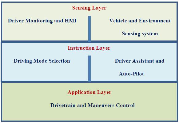
The instruction layer holds high-level programs for longitudinal and lateral vehicular control, including speed, acceleration, road profile, and direction. After considering such parameters, the computed optimum data will be communicated through the intra-vehicle network to the vehicle powertrain. Feedback regarding the action taken is returned for further optimization.
The instruction layer provides necessary commands to the application layer regarding actions required to achieve optimal stability and comfort. The application layer actively and dynamically exchanges data and affects the powertrain operations related to vehicle movements and trajectories. This can all be carried out automatically and intelligently in the autonomous vehicle environment, ensuring the safety and reliability of the travelled journey and balancing between handling, stability and comfort [20].
Due to the recent development in the automotive industry and vehicular control and computing power, using optimization, simulation, and intelligent algorithms, focus on the vehicle suspension design for both comfort and handling become possible using techniques ranging from numerical analysis to simulation of vehicular operations [21-23]. Active and semi-active suspension systems for automotive applications are designed and tested using mechatronics systems. Sensors and actuators are used within the vehicle control environment to enable higher safety and optimum comfort levels [24-27].
This paper aims to establish a selection strategy for driving mechanisms in autonomous vehicles as a function of both road profile and tire and suspension springs interaction in order to achieve either optimum handling and/or optimum comfort and will establish criteria for a selection that presents good comfort and good handling, which deals with both longitudinal and vertical dynamics.
2. MATERIALS AND METHODS
For the suspension system of the vehicles, especially autonomous ones, to perform optimally over different road profiles with different roughness and elevations and to enable road better road handling to ensure safety, variable stiffness to damping ratios need to be considered in selecting driving mode automatically by the self-driving vehicle. This reliable approach provides a mechanism to optimize vehicle movement based on road profile and speed [28-32].
A Quarter Car Model simulation is carried out with the following considerations to achieve this research work objectives, with Table 1 presenting symbols/acronyms and their meaning [33, 34]:
(1) Different suspension stiffness to damping ratios over three levels of road profile are carried out at a speed of 60Km/h, considered the average driving speed that could be used both inside a city and on highways.
(2) Tire spring length and Suspension spring length variations in response to road profile and suspension stiffness to damping ratios.
(3) Sprung Mass Acceleration at three levels of road profile.
| Symbols/Acronyms | Meaning |
| UMRP | Un-sprung Mass Reference position. |
| TSRP | Tire Spring Reference Position. |
| E | Road Elevation. |
| v | Vehicle Speed. |
| k | Suspension Stiffness coefficient. |
| c | Damping Coefficient. |
| SMRP | Sprung Mass Reference Position |
| SSRP | Suspension Spring Reverence Position. |
| SLVR | Spring Length Variation. |
| SMA | Sprung Mass Acceleration. |
| SMP | Sprung Mass Position. |
| Ls (Tire) | Tire Spring Length |
| Ls (Suspension) | Suspension Spring Length |
Ls (Tire) is computed according to equation (1), with Ls (Suspension) computed as in equation (2).
 |
(1) |
 |
(2) |
From Equations (1) and (2), SLVR can be calculated as in equation (3), which correlates the important variables affecting vehicle driving in terms of comfort, handling, and safety.
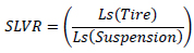 |
(3) |
To further examine the effect of road profile and suspension stiffness on the damping ratio regarding the performance, reliability, handling, and safety of autonomous vehicles, the second derivative in equation (4) is used to evaluate the acceleration of sprung mass as the vehicle travels along a profiled road.
 |
(4) |
This research aims to employ equations (3) and (4) along with the results of the simulations as input to an automatic optimization and selection system that will enable active suspension and tire control, giving autonomous vehicles comfort, safety, and handling. Such a methodology could also be improved, refined, and applied to the design of autonomous cars.
3. RESULTS AND DISCUSSION
Tables 2-4 display MATLAB simulation results for Tire and Suspension Spring length variations as a function of different road profiles that cover different elevations, bumps, and general roughness. The displayed values are noted at a vehicular velocity of 60 km/h. The suspension stiffness to damping ratios is selected to examine and determine both comfort and road handling conditions for smooth and rough roads to enable optimization of design parameters for vehicles' active suspension.
| E=1 | E=3 | E=5 | |||
|
Ls (Tire) |
Ls (Suspension) |
Ls (Tire) |
Ls (Suspension) |
Ls (Tire) |
Ls (Suspension) |
| 0.2508 | 0.4750 | 0.2523 | 0.4750 | 0.2539 | 0.4750 |
| 0.2701 | 0.4515 | 0.3102 | 0.4046 | 0.3504 | 0.3576 |
| 0.2327 | 0.4932 | 0.1981 | 0.5296 | 0.1636 | 0.5660 |
| 0.2735 | 0.4579 | 0.3206 | 0.4236 | 0.3676 | 0.3893 |
| 0.2172 | 0.5105 | 0.1515 | 0.5814 | 0.0859 | 0.6524 |
| 0.2539 | 0.4752 | 0.2618 | 0.4755 | 0.2697 | 0.4758 |
| 0.2740 | 0.4379 | 0.3221 | 0.3637 | 0.3702 | 0.2894 |
| 0.2783 | 0.4488 | 0.3348 | 0.3964 | 0.3913 | 0.3441 |
| 0.2239 | 0.5006 | 0.1717 | 0.5519 | 0.1195 | 0.6032 |
| 0.2966 | 0.4251 | 0.3898 | 0.3252 | 0.4831 | 0.2254 |
| 0.2479 | 0.4815 | 0.2436 | 0.4945 | 0.2394 | 0.5075 |
| 0.2508 | 0.4847 | 0.2524 | 0.5040 | 0.2540 | 0.5234 |
| 0.2253 | 0.5085 | 0.1758 | 0.5754 | 0.1263 | 0.6423 |
| 0.2698 | 0.4535 | 0.3094 | 0.4105 | 0.3490 | 0.3675 |
| 0.2630 | 0.4627 | 0.2890 | 0.4382 | 0.3151 | 0.4137 |
| 0.2552 | 0.4695 | 0.2657 | 0.4585 | 0.2761 | 0.4475 |
| 0.2869 | 0.4405 | 0.3606 | 0.3715 | 0.4344 | 0.3025 |
| 0.2219 | 0.5135 | 0.1658 | 0.5904 | 0.1097 | 0.6674 |
| 0.2757 | 0.4614 | 0.3270 | 0.4343 | 0.3783 | 0.4072 |
| 0.2437 | 0.4936 | 0.2312 | 0.5307 | 0.2187 | 0.5679 |
| 0.2393 | 0.4945 | 0.2178 | 0.5335 | 0.1964 | 0.5725 |
| E=1 | E=3 | E=5 | |||
|
Ls (Tire) |
Ls (Suspension) |
Ls (Tire) |
Ls (Suspension) |
Ls (Tire) |
Ls (Suspension) |
| 0.2508 | 0.4750 | 0.2523 | 0.4750 | 0.2539 | 0.4750 |
| 0.2724 | 0.4486 | 0.3171 | 0.3958 | 0.3618 | 0.3429 |
| 0.2263 | 0.4980 | 0.1788 | 0.5441 | 0.1313 | 0.5902 |
| 0.2835 | 0.4469 | 0.3505 | 0.3906 | 0.4175 | 0.3344 |
| 0.2024 | 0.5251 | 0.1073 | 0.6254 | 0.0122 | 0.7257 |
| 0.2713 | 0.4588 | 0.3139 | 0.4265 | 0.3566 | 0.3941 |
| 0.2619 | 0.4508 | 0.2856 | 0.4023 | 0.3094 | 0.3538 |
| 0.2885 | 0.4346 | 0.3654 | 0.3537 | 0.4424 | 0.2728 |
| 0.2077 | 0.5149 | 0.1231 | 0.5947 | 0.0385 | 0.6745 |
| 0.3219 | 0.3953 | 0.4657 | 0.2359 | 0.6096 | 0.0766 |
| 0.2159 | 0.5078 | 0.1476 | 0.5735 | 0.0793 | 0.6392 |
| 0.2828 | 0.4477 | 0.3483 | 0.3931 | 0.4138 | 0.3385 |
| 0.1909 | 0.5400 | 0.0727 | 0.6700 | 0.0455 | 0.8000 |
| 0.3085 | 0.4128 | 0.4256 | 0.2885 | 0.5426 | 0.1642 |
| 0.2254 | 0.4963 | 0.1762 | 0.5390 | 0.1270 | 0.5817 |
| 0.2883 | 0.4324 | 0.3648 | 0.3473 | 0.4414 | 0.2621 |
| 0.2617 | 0.4595 | 0.2851 | 0.4286 | 0.3085 | 0.3977 |
| 0.2338 | 0.4957 | 0.2015 | 0.5372 | 0.1692 | 0.5786 |
| 0.2755 | 0.4573 | 0.3266 | 0.4219 | 0.3777 | 0.3865 |
| 0.2351 | 0.4986 | 0.2052 | 0.5457 | 0.1754 | 0.5929 |
| 0.2524 | 0.4799 | 0.2572 | 0.4898 | 0.2619 | 0.4997 |
| E=1 | E=3 | E=5 | |||
|
Ls (Tire) |
Ls (Suspension) |
Ls (Tire) |
Ls (Suspension) |
Ls (Tire) |
Ls (Suspension) |
| 0.2508 | 0.4750 | 0.2523 | 0.4750 | 0.2539 | 0.4750 |
| 0.2654 | 0.4575 | 0.2963 | 0.4225 | 0.3271 | 0.3875 |
| 0.2442 | 0.4849 | 0.2325 | 0.5047 | 0.2209 | 0.5246 |
| 0.2606 | 0.4729 | 0.2818 | 0.4688 | 0.3030 | 0.4646 |
| 0.2324 | 0.4938 | 0.1971 | 0.5313 | 0.1618 | 0.5688 |
| 0.2398 | 0.4857 | 0.2195 | 0.5071 | 0.1992 | 0.5285 |
| 0.2719 | 0.4375 | 0.3156 | 0.3624 | 0.3593 | 0.2873 |
| 0.2837 | 0.4512 | 0.3510 | 0.4035 | 0.4183 | 0.3559 |
| 0.2348 | 0.4961 | 0.2043 | 0.5382 | 0.1739 | 0.5803 |
| 0.2729 | 0.4537 | 0.3188 | 0.4111 | 0.3646 | 0.3685 |
| 0.2725 | 0.4668 | 0.3175 | 0.4503 | 0.3625 | 0.4338 |
| 0.2397 | 0.5015 | 0.2191 | 0.5546 | 0.1985 | 0.6077 |
| 0.2334 | 0.4991 | 0.2001 | 0.5472 | 0.1668 | 0.5953 |
| 0.2547 | 0.4647 | 0.2642 | 0.4442 | 0.2737 | 0.4237 |
| 0.2724 | 0.4545 | 0.3171 | 0.4134 | 0.3619 | 0.3723 |
| 0.2552 | 0.4732 | 0.2656 | 0.4696 | 0.2759 | 0.4659 |
| 0.2798 | 0.4533 | 0.3393 | 0.4098 | 0.3988 | 0.3664 |
| 0.2420 | 0.4996 | 0.2259 | 0.5489 | 0.2098 | 0.5981 |
| 0.2533 | 0.4845 | 0.2600 | 0.5035 | 0.2667 | 0.5224 |
| 0.2584 | 0.4772 | 0.2753 | 0.4816 | 0.2922 | 0.4859 |
| 0.2339 | 0.4953 | 0.2016 | 0.5360 | 0.1694 | 0.5767 |
| k:c=0.25 | k:c=0.2 | k:c=0.17 | |||
|
Ls (Tire) |
Ls (Suspension) |
Ls (Tire) |
Ls (Suspension) |
Ls (Tire) |
Ls (Suspension) |
| 0.2539 | 0.4750 | 0.2539 | 0.4750 | 0.2539 | 0.4750 |
| 0.3255 | 0.3896 | 0.3198 | 0.3969 | 0.3150 | 0.4032 |
| 0.2243 | 0.5222 | 0.2363 | 0.5142 | 0.2459 | 0.5080 |
| 0.3003 | 0.4681 | 0.2921 | 0.4788 | 0.2869 | 0.4860 |
| 0.1642 | 0.5655 | 0.1709 | 0.5554 | 0.1744 | 0.5484 |
| 0.1973 | 0.5287 | 0.1919 | 0.5275 | 0.1883 | 0.5246 |
| 0.3556 | 0.2900 | 0.3414 | 0.3006 | 0.3285 | 0.3104 |
| 0.4218 | 0.3552 | 0.4342 | 0.3532 | 0.4444 | 0.3528 |
| 0.1775 | 0.5796 | 0.1923 | 0.5765 | 0.2071 | 0.5732 |
| 0.3580 | 0.3762 | 0.3348 | 0.4029 | 0.3158 | 0.4244 |
| 0.3667 | 0.4320 | 0.3787 | 0.4279 | 0.3848 | 0.4266 |
| 0.2001 | 0.6077 | 0.2086 | 0.6037 | 0.2190 | 0.5965 |
| 0.1649 | 0.5951 | 0.1571 | 0.5947 | 0.1501 | 0.5936 |
| 0.2711 | 0.4234 | 0.2610 | 0.4221 | 0.2504 | 0.4213 |
| 0.3626 | 0.3712 | 0.3656 | 0.3668 | 0.3684 | 0.3628 |
| 0.2783 | 0.4649 | 0.2879 | 0.4611 | 0.2975 | 0.4581 |
| 0.3959 | 0.3711 | 0.3862 | 0.3880 | 0.3792 | 0.4023 |
| 0.2155 | 0.5942 | 0.2342 | 0.5818 | 0.2478 | 0.5734 |
| 0.2623 | 0.5265 | 0.2491 | 0.5383 | 0.2404 | 0.5449 |
| 0.2923 | 0.4842 | 0.2897 | 0.4800 | 0.2844 | 0.4782 |
| 0.1713 | 0.5727 | 0.1790 | 0.5572 | 0.1857 | 0.5433 |
Table 5 illustrates further investigation carried out through simulation to establish a point beyond which further changes in the spring ratios (SLVR) will have no effect on the vehicle's overall performance for a specific fixed mechanical at the specified fixed road roughness.
The following are the three cases considered in this work:
A: k:c=1
Figs. (2-4) show the following:
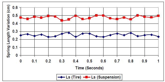
At a smooth road profile with normal elevation and no hard bumps or road holes (E=1), both tire spring and suspension spring vary in parallel but in opposite manner, as shown in Fig. (1). The k:c=1 ratio indicates an un-optimized vehicle condition, where suspension stiffness equals damping.
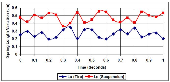
As the road profile is changed to E=3, which includes more road pattern variation, both springs responses, even though they stay as required in terms of polarity, points of crossover and intersection points are observed as presented in Fig. (3). {(0.44, 0.36), (0.47, 0.36)}. The closeness of the springs' responses and the intersection between the curves, in addition to the increase in spring length variation amplitude, indicate the need to optimize the k:c ratio.
The effect of introducing changes in the road profile to simulate stronger road elevation changes (E=5) is presented in Fig. (4). More intersections and higher levels of spring variation are realized due to the need for both springs to exert higher responses to the road profile due to the non-optimized k:c ratio and the higher road profile. {(0.28, 0.34), (0.355, 0.37), (0.43, 0.35), (0.48, 0.36)}. Also, an increase in each spring variation amplitude is realized. Thus k:c=1 is not the optimum setting for (E=5).
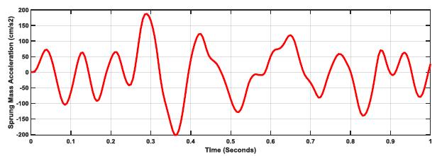
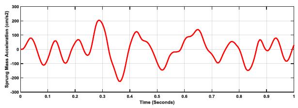
The effect of road profile coupled with the suspension stiffness to damping ratio is further shown in Figs. (5-7), where the Sprung Mass Acceleration (SMA) amplitude increases in response to road profile factor (E) increases but no change in response characteristics. The displayed pattern in the plots reflects the effect of damping on the overall response of the vehicle suspension system as a function of road profile.
B:k:c=20
Fig.s (8-13) show the following:
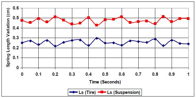
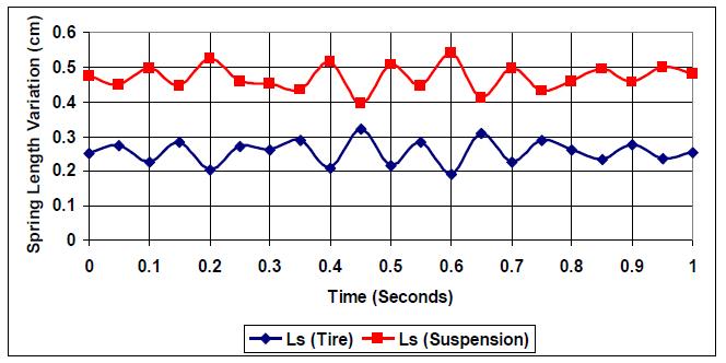
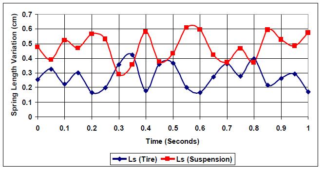
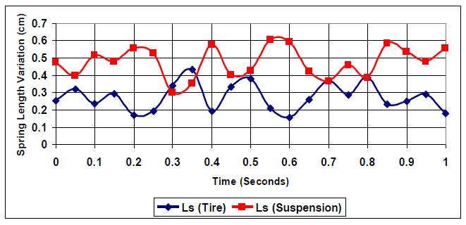
At a smooth road profile with normal elevation and (E=1), tire spring and suspension spring vary in parallel but opposite manner (closer to each other than the case where k:c=1), as shown in Fig. (8). The k:c=20 ratio indicates an optimized vehicle condition, where suspension stiffness is much higher than damping, which reflects a setting for smooth roads and comfortable driving, providing that the road stays at the road profile (E=1).
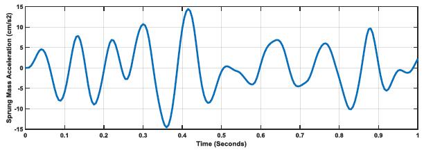
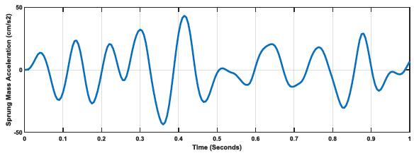
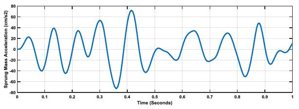
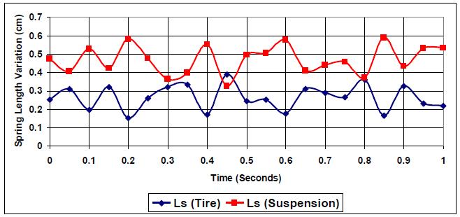
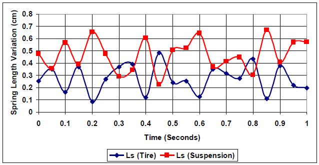
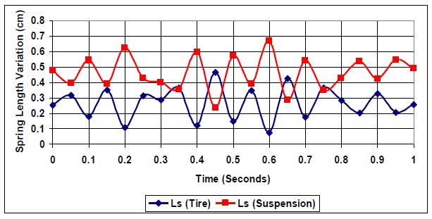
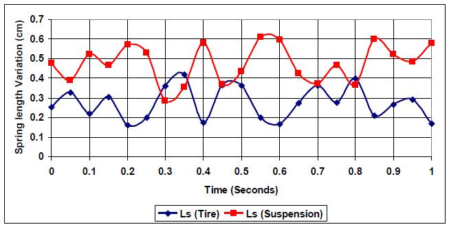
Fig. (9) shows tire and suspension spring responses to road profile (E=3). The curves present a clear intersection between the responses with a higher length variation due to road state. The k:c=20 ratio is designed more for comfort than another driving strategy. This is also illustrated in the number of intersections compared to the case where k:c =1, from two intersection to eight intersections, {(0.33,0.35), (0.35, 0.36), (0.35, 0.43), (0.47, 0.35), (0.64, 0.36), (0.67, 0.36), (0.75, 0.36), (0.77, 0.36)}. The increase in the number of intersections indicates that the vehicle is not tuned correctly for road profile (E=3) as the ratio k:c=20 should be optimized.
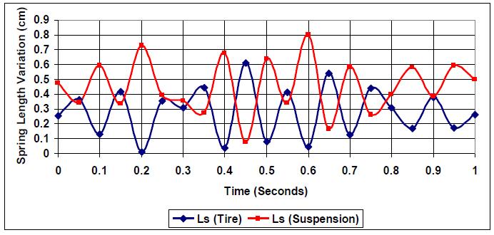
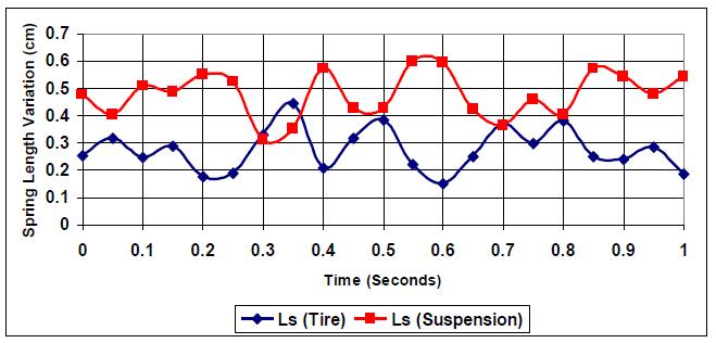
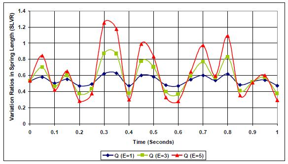
Fig. (10) clearly proves that k:c=20 with E=5, is not a proper optimization for the vehicle, whereby higher levels of spring length variation observed with fourteen intersection points, {(0.04, 0.35), (0.05, 0.35), (0.14, 0.37), (0.16, 0.37), (0.31, 0.33), (0.36, 0.35), (0.43, 0.35), (0.48, 0.35), (0.54, 0.37), (0.56, 0.38), (0.63, 0.38), (0.68, 0.35), (0.74, 0.35), (0.79, 0.35). Thus at this high road profile, k:c:20 will not be effective for such a road profile.
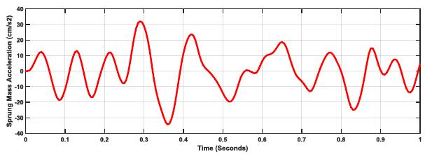
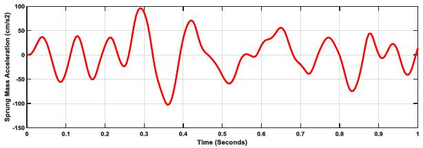
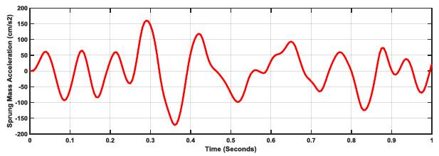
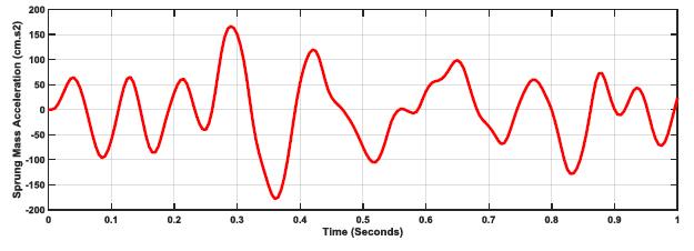
The previous argument is further supported by Figs. (11-13), whereby Sprung Mass Acceleration increases as road profile increases, but with lower values and smoother curves than k:c=1 due to damping. The difference in ratio and the effect of damping as the ratio is moved to k:c=20.
C:k:c = 0.27
Figs (14-19) show the following:
At a smooth road profile with normal elevation (E=1), tire spring and suspension spring vary in parallel but opposite manner (closer to each other than the case where k:c=20), as shown in Fig. (14). The k:c=0.27 ratio indicates an optimized vehicle condition, where suspension stiffness is lower than damping, which reflects a setting for reliable and safe road handling.
Fig. (15) shows tire and suspension spring responses to a road profile (E=3). The curves present a clear indication of the effect of optimizing a vehicle suspension system for rough road conditions as both curves for tire spring and suspension spring stay parallel but much closer compared to the case where (E=1), due to new road condition with length variation close to the smooth road case (R=1). Thus, no intersection at (E=3).
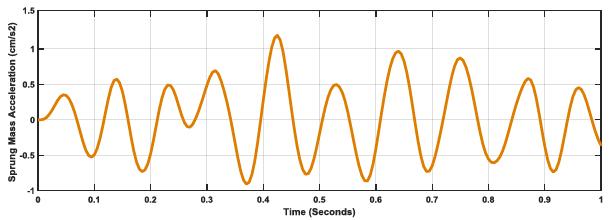
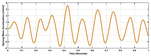
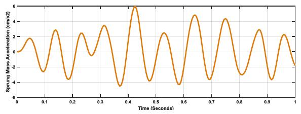
Fig. (16) shows intersection, which are expected at this level of road profile, and when counted found to be six points of intersection, {(0.29, 0.33), (0.36, 0.39), (0.47, 0.37), (0.48, 0.38), (0.78, 0.38), (0.80, 0.38). The number of intersections is less than in the previous cases of k:c=1 and k:c=20. This means that a vehicle suspension ratio optimized using the ratio k:c=0.27 will have better road handling over five profile levels (E from 1 to 5), considering other mechanical coefficients in the design process.
These findings for k:c=0.27 is further supported by the sprung mass acceleration responses for the three considered road profiles, as shown in Figs. (17-19). The plots show the massive difference in acceleration to overcome road profile values and enable safer and more reliable driving through a significant increase in acceleration from E=1 through to E=5.
Further investigation for better optimization with road profile (E=5) is shown in Table 4 and Figs. (20-22), where different k:c values are simulated per the same spring mass, tire stiffness, and speed. The result indicates that the optimized k:c:=0.27 is optimum for handling, slightly improving if the k:c ratio is lowered.
Figs. (20-22) show the obtained four intersection points for:
1. k:c=0.25: {(0.25, 0.325), (0.36, 0.39), (0.79, 0.38), (0.81, 0.385)}
2. k:c=0.2: {(0.29, 0.32), (0.36, 0.395), (0.7, 0.365), (0.8, 0.39)}.
3. k:c=0.17: {(0.3, 0.31), (0.36, 0.4), (0.7, 0.36), (0.71, 0.37}.
It is evident that there is very little change in the spring curves intersection as the k:c values are reduced below 0.27. However, general mechatronic design changes with such simulation could lead to fewer intersection points, reducing the current value from six to four points. (Figs. 23-25) show increased sprung mass acceleration with a reduction in k:c.
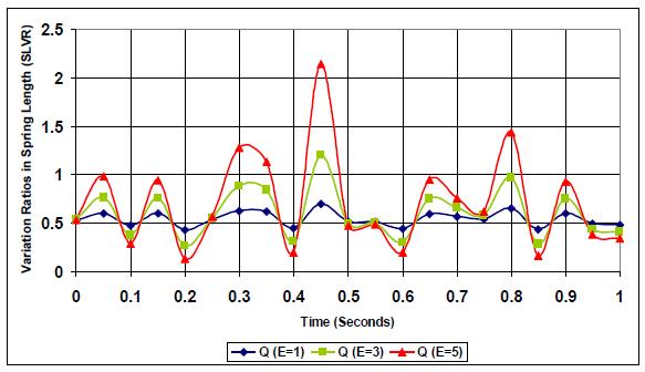
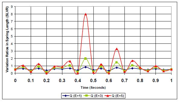
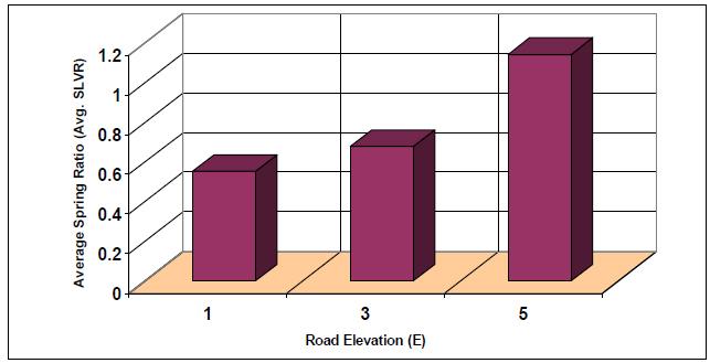
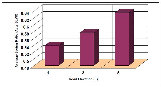
Figs. (26-28) show the equation (3) application to the spring response for both the tire and the suspension systems. It is evident from the plots that the lowest variation ratio (SLVR) is at k;c=0.27 as it is designed for handling different road profiles.
Figs. (29-31) further support this work's findings as it shows the effect of road profile on suspension and tire system performance under different stiffness and damping conditions.
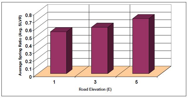
The findings are supported by the presented results in Table 5, where it is evident that for better handling on different road profiles, the Average SLVR ratio describing tire spring and suspension spring variations as a function of road profile and both stiffness and damping per fixed speed, the sprung and un-sprung mass and tire stiffness values should be:
(1) Lower than 1 in value.
(2) Smoothly change in value from low to the high road but not exceeding 1.
Together with sprung mass acceleration and number of intersections, shown in Tables 6 and 8, a three-parameter indicator can be used to enable optimization and driving strategy selection in the design and operation of autonomous vehicles, such that for better handling, the vehicle k:c should be optimized to have a low number of intersections, systematic and proportional increase in MAS, and SLVR less than 1.
| k:c | E=1 | E=3 | E=5 |
| 1 | 0.542 | 0.6 | 0.712 |
| 20 | 0.552 | 0.7 | 1.141 |
| 0.27 | 0.538 | 0.6 | 0.635 |
| k:c | E=1 | E=3 | E=5 |
| 1 | 14 | 40 | 70 |
| 20 | 1.2 | 3.5 | 6 |
| 0.27 | 30 | 100 | 150 |
| k:c | E=1 | E=3 | E=5 |
| 1 | 0 | 2 | 4 |
| 20 | 0 | 8 | 14 |
| 0.27 | 0 | 0 | 6 |
CONCLUSION
This work uses MATLAB simulation to establish criteria for optimization of vehicle-road interaction through varying road profiles and suspension stiffness to damping ratios. The work presented a new technique to optimize comfort and handling, using the intersection between tire spring and suspension spring length variation and analysing the subsequent sprung mass acceleration. The work considered a vehicle speed of 60km.h needs to further consider other velocities and different sprung and un-sprung mass parameters, various tire stiffness and a wider range of road profiles to enable a reliable automatic control system to select driving mode as per road profile and function of vehicle parameters. Vehicle design and development now include simulation of vehicle models on a regular basis, which not only shortens the time it takes to go from concept to production but also saves money and time over prototyping. Additionally, it enables performance optimization to create safer cars with the best handling and ride comfort features that can be automatically modified depending on the road profile by autonomous and intelligent cars. Using an integrated strategy, driving comfort, vehicle handling, and suspension control enable an autonomous vehicle to select the ideal mode of driving as a function of road profile.
Intelligently matching road profiles with speed and the vehicle suspension system in autonomous vehicles can effectively contribute to safety enhancement and accident reduction. Thus, a switching mechanism per road profile can be implemented based on the simulated characteristics at the three levels of road profile and different suspension stiffness to damping coefficients.
CONSENT FOR PUBLICATION
Not applicable.
AVAILABILITY OF DATA AND MATERIALS
The authors confirm that the data supporting the findings of this study are available within the manuscript.
FUNDING
None.
CONFLICT OF INTEREST
The author declares no conflicts of interest, financial or otherwise.
ACKNOWLEDGEMENTS
This MATLAB program used in this work was written by James T. Allison, Assistant Professor at the University of Illinois at Urbana-Champaign.

