All published articles of this journal are available on ScienceDirect.

Projecting the Impact of New Public Transport Networks on Mode Shift
Abstract
Background:
Although many studies have identified the key factors influencing travel mode, they have typically centred around survey data, which has several limitations. In this research, actual transport data (GPS) has been provided by Google Environment Insights Explorer (EIE) for 169 municipalities in Australia across 2018 and 2019.
Objective:
A key outcome of this paper is to project the independent impact of new public transport networks (rail, bus and tram) on mode shift away from vehicles for each municipality and estimate the total distance travelled.
Methods:
This study uses a combination of linear regression and logit transformations to predict the proportion of automobile transport relative to all other transport modes.
Results:
The results suggest that South Australia would benefit from a metropolitan northeast rail line, New South Wales would benefit from a metropolitan southwest tram line, and Victoria would benefit from a metropolitan southeast bus service.
Conclusion:
Although the analysis is somewhat crude, it utilises open-access data and thus could be easily replicated for any country globally, which could be greatly beneficial, especially for countries with low socio-demographic backgrounds.
1. INTRODUCTION
Transport issues in Australia have been an ongoing point of conjecture due to growth in the major cities which has led to increases in commuting times and greenhouse gas emissions [1]. Melbourne and Sydney, the capitals of Victoria and New South Wales, respectively, have both released ‘Plan Melbourne’ [2] and ‘Greater Sydney Region Plan: A Metropolis of three Cites’ [3], which are planning strategies to 2050 and beyond. The central premise of both of these strategies is the idea of living locally whereby in Melbourne, we create ‘20 minute neighbourhoods’, and Greater Sydney is decentralised and transformed into a metropolis of three cities, namely Western Parkland City, Central River City and Eastern Harbour City. A key component of ‘Plan Melbourne’ [2] is building better transport infrastructure and services in newer suburbs, including new bus services for outer suburbs and expansions to the rail network where there is sufficient demand. This highlights the importance of demand modelling of public transport and or projecting the impact this has on mode shift away from vehicle transport.
1.1. Research Gap
Numerous studies have examined trends in mode share in Australian cities. Census data to investigate the relationship between distance from CBD and the number of cars per household to see what impact these had on active transport mode share [4]. A key finding was that the relationship between distance to CBD and active transport mode share was weak. However, they assumed the relationship between distance to CBD and active transport mode share is linear, which it was not as there appeared to be a very strong non-linear trend. They also used levels of car ownership per household as a proxy for transport options available and found a strong relationship between active transport usage and the number of cars per dwelling; that is, as the number of cars per dwelling increased, active transport usage decreased. However, it still begs the question of the underlying cause of active mode share as there are many reasons why households would have varying levels of car ownership, including distance from CBD and household structure (i.e. number of kids).
Similarly, [1] Pees and Groenhart used Census data and did a longitudinal study of transport mode for Australian capital cities over 35 years. They found public transport usage commenced a revival in 1996 after a rapid decline in the two decades prior. They attribute this increase in transport usage in Melbourne and Sydney to strong total workforce growth (i.e. population). Some of the limitations noted by the authors are that the census data is collected in August when Melbourne tends to be cold and wet, potentially resulting in fewer cyclists and walkers than on a ‘standard’ day. This phenomenon was confirmed by [5], which showed that transport mode choice is seasonal and correlated with temperature.
Stone et al. [6] used spatial data to categorise Local Government Areas (LGA) in Australia into specific regions for each state namely ‘CBD’, ‘CBD Frame’ and ‘Remainder’ to look at the relationship between transport mode and location of the place of work using Census data. This differs from the typical approach of using residential location (or place of origin) to analyse transport mode [1, 4]. They concluded the rise in public transport between 2001 and 2006 was attributed to the dispersal of workplaces away from the inner zone and a greater proportion of these were served by public transport.
Rickwood et al. [7] also looked at Census data to underlying model causes of travel mode share in Australian cities. They acknowledged that a lot of variables (i.e. population density) could be acting as a proxy for the underlying factors influencing public transport mode shares, such as proximity to CBD and public transport accessibility. Several studies have shown distance to public transport strongly linked to transport modal choice, including [8, 9].
To date, much research around transport mode has focused predominantly on Census data and survey data in general. One of the key benefits of survey data is it enables modelling of mode choice behaviour at the individual level, which isn’t possible with big data due to privacy reasons. However, survey data is available infrequently and costly. Furthermore, survey data only provides information on the primary mode of transport for a single day of the year for work-related travel. [10] states that with big new data sources available, including phone call data records, this allows us to observe and understand mobility behaviour in unprecedented detail. Several studies have used mobile phone and GPS data to detect transport mode [11, 12] and estimate travel activity patterns [13-15] Although there have been studies in Australia using GPS data to model transport behaviour these are generally limited to a small subset of respondents using GPS tracking [16, 17]. To the best of the authors’ knowledge, there has been no large-scale study in Australia using GPS data, specifically mobile phone data, to model transport behaviour.
Milne and Watling [18] discussed the potential limitations of big data in the context of planning transport systems, including data ownership and suggested that although the volume of data might increase, the granularity is likely to decrease around mode, vehicle type, vehicle occupancy, journey purpose and various demographic features. They also suggest that based on current trends, automatically recorded digital data will inevitably become mainstream for academic study and the practical planning of transport systems. This is due to the many benefits, including reductions in time/cost and improvements in repeatability and scalability. They propose using big data to gain new insights rather than replacing it for survey data using the existing applications. This is supported by [19], who, amongst other things, surveyed professional planners about the anticipated changes over the next ten years. One of the key themes was data-driven future with new sources of data and insights.
1.2. Article Outline
In this research, Google Environment Insights Explorer (EIE) data is used to model transport mode, and this overcomes many of the shortcomings in the literature as it incorporates all modes of transport for a single journey rather than just the primary mode of transport, which is standard in survey data. Furthermore, the EIE data is aggregated on an annual basis and is not biased in the same way the Census data is, which is based on travel behaviour for a single day and thus could be heavily influenced by the weather on that day. Also, the EIE data incorporates all reasons for travel above and beyond work-related travel. This EIE data is then used to quantify the independent impact of the availability of each public transport mode (tram, rail and bus) on mode shift away from vehicle transport controlling for all other variables for Australian municipalities. Integrating the total distance travelled based on EIE data makes it possible to project the impact of any new public transport system, which is a novel insight and significant contribution to the literature and transport planning in general.
2. MATERIALS AND METHODS
The Google Environmental Insights Explorer (EIE) is a free tool developed by Google which showcases building emissions, transport emissions and rooftop solar potential for cities globally. The EIE data which is used to derive the transport emissions incorporates actual distance travelled (kms) at the individual municipality level, which is then aggregated across regions and years and broken down by boundary (inbound, outbound and in boundary) and transport mode (automobiles, motorcycles, bus, rail, tram, walking and cycling). National Greenhous Gas Inventory and Snapshot Climate [20, 21] have more information regarding transport emissions in Australian states and municipalities.
For simplicity, the transport mode is grouped into three specific sectors, namely vehicles (automobiles and motorcycles), public transport (bus, rail and tram) and active transport (walking and cycling). Since one municipality's inbound data is another municipality's outbound data, it is important to divide inter-municipality data (inbound and outbound) by two to avoid double counting. The total distance travelled for all transport modes for each municipality i for year j is defined in equation 1.
 |
(1) |
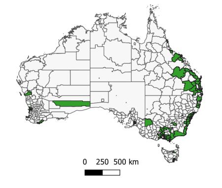
Australia is divided into 7 different states and territories namely New South Wales (NSW), Victoria (VIC), Queensland (QLD), South Australia (SA), Western Australia (WA), Tasmania (TAS), Northern Territory (NT) and Australian Capital Territory (ACT). It is quite a large country with a total land area of 7.692 million km2 [22]. However, the bulk of the population is concentrated in Victoria and New South Wales (59%) even though they only make up (13%) of the national land area [23]. EIE data is anonymous and highly aggregated and primarily based on the same underlying information made available in Google Maps [24]. There are a total of 537 municipalities in Australia and EIE data has been provided for 169 of these municipalities across 2018 and 2019. The main reason there is no completeness in the EIE data for all municipalities is there is not enough data to meet a minimum threshold for privacy protections. It is important to note that the capital city of each state and territory is also missing due to inconsistencies with the boundary definitions of these regions.
Fig. (1) displays the geographical location of these municipalities where the EIE data is present.
EIE data is predominantly present for metropolitan municipalities, excluding capital cities nationwide, however, there are several anomalies. For example, Kalgoorlie in Western Australia is a very large municipality measuring 95,498km2 with a population of 29,469, which is located 595km from the capital Perth. Conversely, Warrnambool in Victoria is a very small municipality measuring 121km2 with a population of 35,181 which is located 265km from the capital Melbourne [22, 23] Therefore, due to the diverse nature of these municipalities outside of the metropolitan areas it was decided to limit all analysis of the EIE data to metropolitan areas as the value of new public transport networks on mode shift is likely to be vastly different for metropolitan areas compared to regional areas. Furthermore, any new public transport station, specifically rail and tram, needs to link to an existing public transport network which may not be possible for many regional municipalities. Fig. (2) displays the geographical location of metropolitan municipalities where EIE data is present for the five major states, namely New South Wales (NSW), Victoria (VIC), Queensland (QLD), Western Australia (WA) and South Australia (SA).
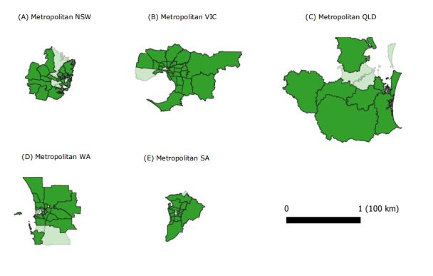
There are 130 metropolitan municipalities across Australia and EIE data is present for 99 of these municipalities, which provides great confidence in completeness. Table 1 displays a breakdown of the provision of EIE data limited to metropolitan municipalities and population in 2019 [23] by state.
The EIE data constitutes 76% of all metropolitan municipalities and these municipalities cover 80% of the total metropolitan population based on 2019 figures providing great confidence in completeness.
Since the geospatial structure of Australia, even limited to the metropolitan regions is diverse, it is important to first analyze the EIE data on a state-by-state metropolitan basis as this might impact how the EIE data is modelled. Table 2 displays the total distance broken down by transport mode for each state for 2018 and 2019 combined, limited to metropolitan municipalities.
Interestingly, public transport usage is highly correlated with the population figures in Table 1. This is not surprising given the public transport networks are likely to differ vastly within each state. The bigger states like NSW and VIC can support a more frequent public transport system relative to other states due to their respective population. Table 3 displays the Total Distance based on equation 1 broken down by public transport mode for each state for 2018 and 2019 combined.
| State | LGA’s (Total) | LGA’s (EIE) | Population (Total) | Population (EIE) |
|---|---|---|---|---|
| VIC | 31 | 29 (94%) | 4,999,184 | 4,549,742 (91%) |
| NSW | 30 | 24 (80%) | 4,768,575 | 3,560,608 (75%) |
| QLD | 9 | 8 (89%) | 3,200,172 | 1,946,190 (61%) |
| SA | 19 | 15 (79%) | 1,311,130 | 1,231,738 (94%) |
| WA | 30 | 19 (63%) | 1,982,315 | 1,782,513 (90%) |
| TAS | 5 | 3 (60%) | 216,410 | 144,086 (67%) |
| NT | 6 | 1 (17%) | 68,636 | 38,270 (56%) |
| Total | 130 | 99 (76%) | 16,546,422 | 13,253,147 (80%) |
Table 2.
| State | Vehicle Transport | Public Transport | Active Transport |
|---|---|---|---|
| VIC | 53,412 (87.8%) | 5,869 (9.7%) | 1,532 (2.5%) |
| NSW | 36,556 (80.3%) | 7,636 (16.8%) | 1,317 (2.9%) |
| QLD | 25,863 (95.7%) | 793 (2.9%) | 380 (1.4%) |
| SA | 14,062 (94.9%) | 420 (2.8%) | 334 (2.3%) |
| WA | 21,714 (93.4%) | 1,095 (4.7%) | 429 (1.8%) |
| TAS | 1.632 (97.2%) | 19 (1.1%) | 29 (1.7%) |
| NT | 302 (99.1%) | 0 (0.0%) | 3 (0.9%) |
| Total | 153,542 (88.5%) | 18,749 (9.1%) | 5,250 (2.3%) |
| State | Bus | Rail | Tram |
|---|---|---|---|
| NSW | 1,118 (14.6%) | 6,505 (85.2%) | 13 (0.2%) |
| VIC | 435 (7.4%) | 4,618 (78.7%) | 815 (13.9%) |
| QLD | 70 (8.8%) | 641 (80.8%) | 83 (10.5%) |
| SA | 183 (43.4%) | 205 (48.8%) | 33 (7.8%) |
| WA | 179 (16.4%) | 916 (83.6%) | 0 (0.0%) |
| NT | 0 (0.0%) | 0 (0.0%) | 0 (0.0%) |
| TAS | 19 (100.0%) | 0 (0.0%) | 0 (0.0%) |
| Total | 2,003 (12.6%) | 12,885 (81.4%) | 944 (6.0%) |
Rickwood et al. [7] used a dummy variable for each state and territory when predicting transport mode to account for the diverse geospatial structure of each state and territory. Interestingly, the coefficients for the independent variables (distance to CBD, population density and cars per household) were similar to a Sydney-based model once dummies for states were included. Due to small sample sizes and the desire to focus on similar metropolitan regions, Northern Territory (NT) and Tasmania (TAS) have been excluded from all future analysis.
2.1. Exploration
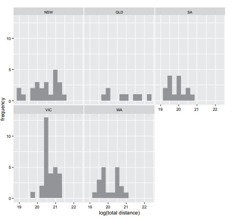
Fig. (3) displays a histogram of Total Distance defined in equation 1 split by each state limited to the metropolitan regions. A natural log transformation was applied to Total Distance due to the distribution of the data to ensure normality.
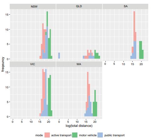
Interestingly, Western Australia and South Australia are the only states with somewhat similar distributions of the five major states. New South Wales and Victoria are often comparable states due to their land size and population, but their distribution of Total distance is vastly different. Victoria has far more municipalities concentrated around the mean, whereas New South Wales has a greater spread of municipalities with very small Total distance (Lane Cove, Mosman and Burwood) and less concentration around the mean. Queensland appears to be unique, with several large outliers, including Gold Coast, a major city. Fig. (4) shows a histogram of Total Distance split by mode type (vehicle transport, public transport and active transport).
Interestingly, Victoria and New South Wales are much more comparable when split by transport mode. Similarly, to Fig. (3) South Australia and Western Australia are comparable, and Queensland is quite unique in terms of the distribution of total distance by transport mode. The distribution of public transport for Queensland is particularly interesting considering there is very little concentration around the mean, suggesting large variance in public transport usage by individual municipalities in Queensland.
There is some evidence that the states should not be modelled collectively since the distribution of total distance for each state and territory varies considerably. However, due to small sample sizes and the potential of overfitting, the same approach as [7] is applied using dummy variables for each state to account for the diverse idiosyncrasies within each state and territory. New South Wales is used as the ‘base’ state since it has the smallest proportion of automobile transport and many metropolitan municipalities, so there is no dummy variable for New South Wales.
3. ANALYSIS
Several studies have used logistic regression to predict travel mode [9, 25-27]. However, these studies use survey data where each travel mode's outcome variable is individual responses (binary). In this research, it is not possible to use logistic regression since the outcome variable is the aggregated proportion of each travel mode and is thus non-binary. In statistics, any proportion is bounded between 0 and 1. Therefore, linear regression cannot be applied directly to the proportion of each transport mode, as it is possible for the predicted values to fall outside these ranges. It is therefore, important a data transformation is applied. Rickwood and Glazebrook [7] used a variation of an arcsine transformation which means the scale goes from (0,1) to (0,ð) and the relationship between p and arcsine(p) becomes non-linear, especially as p approaches 0 and 1. However, arcsine(p) is still bounded by (0,ð/2), so it is still possible to have predicted probabilities below 0 and above 1.
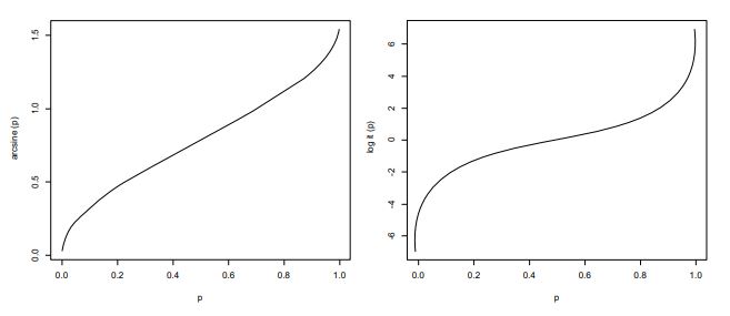
This study [28] shows how to model proportions by integrating a logit transformation on the dependent variable and then using linear regression. This method ensures the predicted proportions are bounded by 0 and 1 since a logit transformation is effectively unbounded. However, the predicted proportions must lie within the unit interval (0,1) but not equal to 0 or 1 as a logit transformation is not defined for these values. A similar approach to [28] is applied in this research. Equation 2 displays the logit transformation calculations.
 |
(2) |
Equation 3 shows how to convert the logit value back into probabilities.
 |
(3) |
To give some context Fig. (5) displays the arcsine and logit transformation.
There are three different transport modes: vehicles, public transport and active transport. So, there are potentially three different models for each transport mode, but considering vehicle transport constitutes 88.5% of all transport, this is the key one to focus on since governments and planning authorities are typically interested in shifting transport modes from vehicles to public transport and active transport. Also, in the EIE data, no municipality had 100% (or 0%) vehicle transport, so no undefined values were using a logit transformation.
The proportion of vehicle transport is modelled nationally using stepwise linear regression and a p-value of 0.001 as the cut-off to find the underlying cause of transport mode. A logit transformation is also applied to the dependent variable based on equation 2 and dummy variables are used for all states, excluding New South Wales, which is the ‘base’ state. Additional dummy variables are included for each public transport option namely ‘rail’, ‘tram’ and ‘bus’ based on whether there was non-zero EIE data for this mode type for each municipality to quantify their individual importance controlling for all public transport modes.
In this study they [29] found that although many people assume Australia’s major cities are monocentric, that is, most workers converge on the CBD for their work. The reality is this only represents around 15% of the population, whereas approximately 75% of jobs are randomly dispersed throughout the city. Furthermore, they also found that workers don’t live very far from where they work, which has changed little over time. This phenomenon is also found in the United States metropolitan areas where suburb-to-suburb commuting represents 40% of the total journey-to-work trips [30]. Therefore, in this research, distance to CBD is included as a pseudo measure for representing people whose commuting behaviour is intra-suburban where public transport is less viable for their transport needs. It is important to include this measure since any new public transport network is likely to be built on the fringe of the metropolitan area and without this measure the analysis would likely overstate the importance of a new public transport network. Other studies have used distance to the CBD as pseudo measures, including [7], which generally used it to represent how accessible a local transit stop is to employment destinations.
Distance to CBD was calculated using the QGIS software based on the distance between the centroid of each municipality and their respective capital city [31] and a natural log transformation was applied to ensure normality. Equation 4 shows the model formulation and Table 4 shows the stepwise linear regression model results.
Table 4.
| Variable | Coefficient (t-stat) | R2 |
|---|---|---|
| Intercept | 1.288 (5.199) | 0.809 |
| RAIL | -0.786 (-7.044) | - |
| BUS | -0.404 (-3.600) | - |
| TRAM | -0.307 (-3.157) | - |
| DIST | 0.458 (8.153) | - |
| VIC | 0.650 (6.685) | - |
| QLD | 1.238 (8.053) | - |
| SA | 1.477 (12.831) | - |
| WA | 1.295 (13.437) | - |
 |
(4) |
Where
VEHi,j = Proportion vehicle transport relative to all other transport modes for municipality i in year j
RAILi,j = Binary variable to denote non-zero Rail EIE data for municipality i in year j
TRAMi,j = Binary variable to denote non-zero Tram EIE data for municipality i in year j
BUSi,j = Binary variable to denote non-zero Bus EIE data for municipality i in year j
VICi = Binary variable to denote if municipality i is in Victoria
QLDi = Binary variable to denote if municipality i is in Queensland
SAi = Binary variable to denote if municipality i is in South Australia
WAi = Binary variable to denote if municipality i is in Western Australia
The results suggest that of the three public transport options available, rail is by far the most important, followed by buses then trams in terms of impacting the proportion of vehicle travel mode controlling for all other variables. It is also important to note that a new bus network is likely to be significantly cheaper than a new tram (and rail) network due to less infrastructure requirements. Interestingly [32], found car users in Porto to have a highly positive view of light rail (trams) relative to buses due to perceived comfort, reliability, transport status and ambiance, even though it was more expensive and had less coverage relative to bus networks. This suggests the perception of public transport options in Australia may need further consideration when planning public transport networks. Also, the binary variable for each state supports the results in Table 2 where New South Wales had the lowest proportion of vehicle transport followed by Victoria and South Australia, Queensland and Western Australia were all comparable.
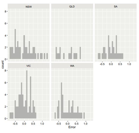
Fig. (6) displays a histogram of the residuals split by state. The residuals are defined as the residuals of the regression model defined in equation 4, not the estimated proportions' residuals. Interestingly, most of the outliers are in New South Wales and are predominantly inner-city municipalities, including Strathfield, Burwood and North Sydney, with extremely high levels of public transport use.
4. RESULTS AND DISCUSSION
All metropolitan municipalities in Australia have at least one public transport option (rail, tram or bus) available. Therefore, a hypothetical municipality will be used to gauge the impact of a new public transport network and calculate the estimated total distance. These calculations are derived using the coefficients for each public transport option in Table 4 and the formulas in Equations 2 and 3. Suppose the hypothetical municipality had a Total Distance of 500,000,000kms and the proportion of vehicle transport was 98%. Table 5 shows the results.
These calculations can be applied to all municipalities across all years to gauge where the greatest impact of ofimplementing a new tram, bus or rail network lies. It is important to note that although EIE data may be present for a specific municipality, it may be missing for a specific transport mode (specifically public transport) within that municipality due to not meeting a minimum privacy threshold. Table 6 shows the top 10 municipalities nationwide for a new rail network ranked according to the projected total distance.
| New Public Transport Mode | Vehicle Proportion New | Projected Distance |
|---|---|---|
| Rail | 95.7% | 11,424,060 |
| Bus | 97.0% | 4,835,568 |
| Tram | 97.3% | 3,499,697 |
| State | Municipality | Vehicle Proportion | Vehicle Proportion adj | Projected Distance |
|---|---|---|---|---|
| SA | West Torrens | 95.5% | 90.6% | 26,070,687 |
| SA | Tea Tree Gully | 95.8% | 91.2% | 23,513,305 |
| SA | Norwood Payneham St Peters | 94.2% | 88.1% | 17,124,739 |
| QLD | Noosa | 97.3% | 94.3% | 15,670,028 |
| SA | Burnside | 94.9% | 89.4% | 14,522,204 |
| SA | Campbelltown | 94.2% | 88.0% | 13,538,279 |
| WA | Belmont | 97.9% | 95.5% | 11,790,762 |
| SA | Adelaide Hills | 97.2% | 94.0% | 10,642,820 |
| WA | Kalamunda | 98.3% | 96.4% | 7,249,107 |
| QLD | Scenic Rim | 99.3% | 98.4% | 3,917,731 |
| State | Municipality | Vehicle Proportion | Vehicle Proportion adj | Projected Distance |
|---|---|---|---|---|
| QLD | Moreton Bay | 94.9% | 92.6% | 70,543,054 |
| VIC | Casey | 92.7% | 89.4% | 61,496,750 |
| VIC | Yarra Ranges | 93.4% | 90.4% | 38,354,349 |
| QLD | Ipswich | 95.9% | 93.9% | 27,636,418 |
| VIC | Cardinia | 93.0% | 89.8% | 24,737,066 |
| VIC | Mornington Peninsula | 97.6% | 96.4% | 18,525,030 |
| NSW | Camden | 94.0% | 91.2% | 14,726,094 |
| WA | Armadale | 94.6% | 92.1% | 10,491,221 |
| QLD | Scenic Rim | 99.3% | 98.9% | 1,644,159 |
| WA | Mundaring | 99.0% | 98.5% | 1,381,621 |
| State | Municipality | Vehicle Proportion | Vehicle Proportion adj | Projected Distance |
|---|---|---|---|---|
| NSW | Blacktown | 81.5% | 74.7% | 163,507,013 |
| NSW | Sutherland Shire | 81.1% | 74.2% | 120,344,347 |
| NSW | Cumberland | 74.6% | 66.2% | 115,475,370 |
| NSW | Campbelltown | 78.9% | 71.3% | 96,107,864 |
| NSW | Penrith | 85.6% | 80.0% | 93,606,722 |
| VIC | Monash | 85.3% | 79.5% | 86,630,501 |
| NSW | Northern Beaches | 88.0% | 83.1% | 78,096,071 |
| NSW | Willoughby | 60.0% | 50.0% | 76474699 |
| NSW | Fairfield | 86.4% | 80.9% | 71,466,815 |
| QLD | Moreton Bay | 94.9% | 92.6% | 70,543,054 |
There seems to be strong evidence for a bigger rail system for several inner-city municipalities in Adelaide (South Australia), specifically Tea Tree Gully, Norwood Payneham St Peters and Campbelltown, which are all neighbouring North-East Adelaide municipalities be ideal for a new train line. Table 7 displays the top 10 municipalities for a new bus network ranked according to the projected total distance.
There seems to be solid evidence for a new/expanded bus network in Southeast Victoria, specifically Casey, Yarra Ranges, Cardinia and Mornington Peninsula, all neighbouring suburbs. Several new bus routes were introduced to Casey in 2021 to service the growing communities in Clyde and Clyde North [33]. It is important to note that several municipalities in Table 8 already have a bus network. There are many reasons why a municipality with a bus network might not have corresponding EIE data, including privacy issues and sparse bus schedule data. Also [11], suggests that existing studies using mobile phone network data tend to identify easy-to-detect transport modes (train or metro). Therefore, buses are likely to be harder to classify correctly, considering they share roads with other vehicles and are also a similar size to other road users, including trucks. This suggests current limitations around the bus data, which are likely to improve over time as bus schedule data improves and the precision of the classification of transport modes increases. However, Table 8 displays the top 10 municipalities nationwide for a new tram network ranked according to the projected total distance.
There seems to be strong evidence for a bigger tram system for several inner-city municipalities in Sydney (New South Wales), specifically Blacktown, Sutherland Shire, Cumberland, Campbelltown, Penrith, Fairfield and Liverpool (12th), which are all neighbouring municipalities in South-West Sydney which would be ideal for a new tram line albeit expensive. Also, there has been a commitment from the government to extend the tram network in Monash, Victoria, to connect Monash University and the Chadstone shopping centre [34].
CONCLUSION
The primary outcome of this research is the ability to quantify the impact of different public transport options (rail, bus and tram) on mode shift controlling for distance to CBD and the idiosyncrasies within each state. The results suggest rail was the most important of all public transport options, followed by buses and trams.
This research can be used to determine what impact a new public transport system has on mode shift away from vehicle transport. Furthermore, integrating these results with the total distance travelled for each municipality makes it possible to project the impact (Total Distance) of a new public transport network. These results, alongside the actual costs of new public transport networks, can help councils and governments prioritise new public transport infrastructure.
The analysis, albeit crude, is solely based on freely available data alongside distance to CBD, which can be derived using GIS software. This means that this analysis can be easily replicated in any country globally, which could assist planning authorities, especially those countries with lowsocio-demographic backgrounds. The output of this analysis is not a complete solution for new public transport networks but could be a good starting point for any country to ask further questions about which new public transport networks to integrate and where.
LIST OF ABBREVIATIONS
| LGA | = Local Government Areas |
| EIE | = Environment Insights Explorer |
| NSW | = New South Wales |
| VIC | = Victoria |
| QLD | = Queensland |
| SA | = South Australia |
| WA | = Western Australia |
| TAS | = Tasmania |
| NT | = Northern Territory |
| ACT | = Australian Capital Territory |
CONSENT FOR PUBLICATION
Not applicable.
AVAILABILITY OF DATA AND MATERIALS
The data supporting the findings of the article is available via Google Environmental Insights Explorer at https:// insights.sustainability.google/.
FUNDING
None.
CONFLICT OF INTEREST
The authors declare no conflict of interest, financial or otherwise.
ACKNOWLEDGEMENTS
The authors wish to thank the google environmental insights explorer (EIE) team for their continued support and access to data.

