All published articles of this journal are available on ScienceDirect.

KASSANDRA Model: Detecting Dangerous Traffic Conditions By Modeling Drivers’ Internal Stress Energy
Authors Info & Affiliations
Abstract
Introduction
This paper introduces an innovative method to reduce car accidents by employing mechanical concepts and energy conservation to model drivers’ reactions in unexpected scenarios.
Methodology
The approach involves formulating equations to define drivers’ “internal stress energy,” indicative of their propensity for aggressive driving under time pressure. A spatiotemporal model was developed using traffic data from Highways England and accident data from Transport for London, analyzing around 200 car accidents with data from 80 cameras over two years.
Results and Discussion
Findings suggest a correlation between drivers’ internal stress energy and car accidents, highlighting the predictive value of the proposed equations in assessing road segment dangers. More specifically, using the proposed model with 15-minute timeframes increased car accident prediction four (4) times compared to the evenly spatiotemporal car accident distribution. With smaller timeframes, e.g., two (2) minutes, or with real-time data, its predictive power would be significantly higher!
Conclusion
The equations developed offer a promising tool for estimating and preventing car accidents by modeling the influence of drivers’ stress on driving behavior.
1. INTRODUCTION
Car accident numbers remain high in the 21st century. According to the European Transport Safety Council (ETSC) [1], there was an average of 50 road deaths per 106 inhabitants in the European Union (EU) in 2017. However, only a tiny amount of effort is put into deeply understanding this social problem. It seems that a “normalization” process has taken place [2], and car accidents have been included in societies’ everyday lives. This could be explained using Freud’s repression theory [3] through a normalization process (to feel safe and continue driving).
However, transportation theorists often ignore these parameters and overestimate the need for restricting illegal driving. An illustrative example is the educational campaigns targeting young drivers. These campaigns are usually scientifically grounded on research explaining the factors that lead young drivers to car accidents [4-6], and often indicate that there are psychological factors that result in irresponsible driving. These methods sometimes overestimate drivers’ freedom and personality and, at other times, represent the drivers as deterministically functioning psychological objects [7-10]. This paper highlights that arriving safe depends on how the whole system reacts in unexpected situations.
Quantitative road safety modeling is focused mainly on crash injuries’ severity [11-18] and accident analysis focused on the development and application of advanced econometric and statistical techniques [19]. On the other hand, driver behavior modeling is mainly qualitative [20-23]. Although there were some attempts towards quantitative driver behavior modeling, these were mainly partial models about fatigue, gender, and distracted driving [24-28], stress and risk [29-34], aggressive driving behavior [35-38], dilemma zones at intersections [39-47], car-following [48-57], etc. This paper is a modest proposal toward quantifying driver’s behavior, trying to fill the gap between qualitative and quantitative modeling.
This paper aims to approach drivers’ aggressive behavior in a way that makes it possible to reduce traffic accidents using live data. To do so, a theoretical tool using the energy conservation concept was developed and tested in London Highways. Specifically, drivers are approached as rational agents. Each agent makes an assumption for their arrival time and an expectation for the average velocity they will have during different parts of the journey. Even though this expectation might not be conscious in real life, we believe it determines drivers’ behavior. Our model will suppose that whenever an agent fails to fulfill their expectations, their “internal stress energy” increases, making them drive aggressively. This paper will expand and apply this theoretical tool to London Highways, proving that high spatiotemporal concentrations of internal stress-energy are connected to car accidents. Thus, compared to all the previous approaches mentioned above, the novelty of this research is that it introduces the concept of “internal stress energy” and proves it to be an effective car accident prediction indicator.
We named our approach the “KASSANDRA model” after Cassandra, the daughter of Priam, the King of Troy, whose warnings for disastrous future events were not taken seriously. KASSANDRA is a spatiotemporal model that consists of a set of equations that define drivers’ “internal stress energy,” indicative of their propensity for aggressive driving under time pressure. The findings from the testing of the proposed model suggest a correlation between drivers’ internal stress energy and car accidents, highlighting the predictive value of the proposed model in assessing road segment dangers. The model, its testing, and the findings are presented in the following chapters.
2. METHODOLOGY AND MATHEMATICAL FORMULATION
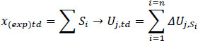
In this paper, we assume that before the start of a journey, each driver has some expectations about its duration. A driver arrives on time at their destination when their location at the expected time is identical to their actual location x(duration)actual=x(duration)expected. However, the drivers’ initial expectations might not be accurate, either because they misinterpreted the conditions before starting or because of unexpected events that occurred during the journey. In this case, they can either change their expectations or try to fulfill them, changing their driving behavior. The main assumption of this paper is that when unexpected events occur, a number of drivers will change their behavior to arrive on time, resulting in car accidents. Therefore, for driver j, we assume that her target is to minimize the difference between her expected and actual journey duration. Equivalently, keeping the duration constant and equal to the expected duration to minimize the difference between her hypothetical location and her actual location. Uj in Eq. (1) represents the utility of the driver at the end of the journey. In Eq. (1), td represents the expected duration of the journey, and v is the velocity of the driver. Throughout the following sections, exp is used to indicate a variable of expected values. If there is no exp indicator, the variable represents the actual conditions.
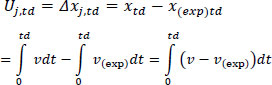 |
(1) |
If the driver arrives at the destination later than the expected time (longer journey than expected), Uj takes negative values. If the driver arrives at the destination before the expected time Uj takes positive values. Even though it is possible to have positive Uj values, this happens when the drivers are free to move with higher velocities than expected. These conditions are not of interest in this paper, which emphasizes drivers who are stressed because they fail to arrive on time. Without loss of generality, we assume that the target of the driver is to maximize Uj.
Eq. (1) represents the utility of the driver j at the end of the journey (t=td). However, throughout the journey, the drivers make estimates and assumptions about the duration of their journey. They often try to assume (consciously or not) if they are going to arrive on time or not. This allows us to define a utility for each driver for every possible time t value (Eq. 2).
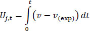 |
(2) |
Next, we move from a temporal to a spatial analysis. Using the derivative of vexp, we get Eq. (3). This is necessary because using road spatial segments instead of temporal sections is more practical.
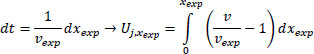 |
(3) |
The journey can be divided into n consecutive segments (S1, S2,..., Sn,) , each with a starting and an ending point. Suppose that xa is the starting point and xb the final point of the segment Si. Then, we can define the variable ∆Uj,Si which represents the utility that the driver gained (or lost) during that segment Si (Eq. 4).
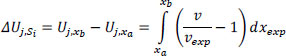 |
(4) |
A negative ∆Uj,Si means that during that segment, the driver was driving slower than their initial expectations, increasing the actual duration of their journey. It goes without saying that Uj,td is the sum of the ∆Uj,Si values (Eq. 5).
 |
(5) |
From the above relationships, we understand that the drivers can increase their utility by adjusting their speed. However, drivers usually cannot unilaterally adjust their speed throughout their journey, as the existence of other drivers affects their behavior. Therefore, j also takes into consideration the velocities of the nearby drivers j. Therefore driver’s j target can be represented using Eq. (6).
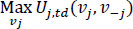 |
(6) |
In this paper, we assume that all drivers perform the same estimations about their journey. This does not indicate that they perform the same journey but that all the drivers expect to find the same driving conditions in each road segment. Even though this assumption limits the findings of this research, it could be considered valid when the drivers are experienced. The reader can find an indicative figure about drivers’ expectations in the appendix. Calculating the hourly average velocities, we can see some spatial and temporal patterns that can be easily guessed/expected by the drivers. The aforementioned assumption makes it possible to create a “hypothetical” driver whose velocity is identical to the hourly average velocity of the drivers of each segment.
We will define the stress-energy of the flow for a road segment {xa, xb} using the classic definition of dynamic energy Energy = mgh, as in Eq. (7):
 |
(7) |
where:
- N: is the number of vehicles in the examined road segment, and
- g: is a constant similar to the gravitational constant representing the inclination of the drivers to change their velocity in order to reach their destination in time.
In this paper, we will assume that every agent has the same g constant, meaning they have the same motivation to reach their destination in time. To avoid examining g, we will define the parameter e in Eq. (8). Examining e is equivalent to examining Energy, as g is a constant. The number of vehicles can be expressed using a density factor: N = ρA, where ρ(vehicles/(m*lanes)) is the car density and A(m*lanes) is the area examined. The number of lanes is expressed using the parameter λ(lanes):
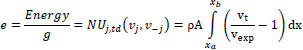 |
(8) |
With the assumption that drivers have similar ∆v in a small part of the road path dx (homogeneity), the integral is simplified for a specific road area (between xa and xb), as follows. The wider the area examined, the more problematic the assumption of homogeneity becomes. Naming L the distance between xa and xb, we get A = λL and from the Eq. (8), we get Eq. (9):
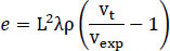 |
(9) |
The higher the e parameter, the more stressed the driver is when she leaves the examined segment (S). We presented a theoretical example to improve the understanding of e. Let us suppose that an unexpected congestion takes place. “Unexpected” means that it does not normally appear at that road segment during that time of the day (visit the appendix for more information about expectations). This congestion will result in lower actual velocity values than expected, resulting in negative internal stress energy values  . The density of the flow (ρ) and the length of the congested segment (L) can worsen the situation, resulting in even more negative internal stress energy values. That stress should be considered an indicator associated with high car accident possibilities. When drivers go through road segments that have high e values, they “collect” energy. However, a car accident is not expected to happen during these parts. We assume that a car accident is expected to occur when energy radically increases or decreases. To find these road parts, we calculate the drivers’ internal “power” (a derivative of e with respect to time t, for a time period {ta, tb}) as shown in Eq. (10):
 |
(10) |
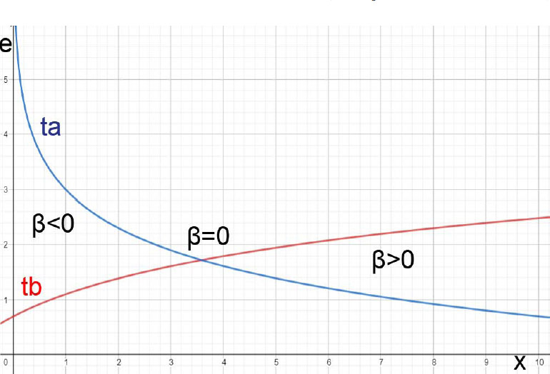
The energy of a road segment decreases in time when β < 0 and increases when β > 0. This means that for a road segment {x1, x2},  for
for  and vice versa. Therefore, supposing that
  for a road segment {x1, x2} and
  for a road segment {x3, x4}, for continuous functions e and β there will be a road segment {x2, s3} in which
  will hold, based on the Bolzano’s theorem.
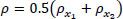
In Fig. (1), we see a group of vehicles with high energy moving from x = 0 to x = 10. As the time variable increases, the energy values of the left road segment decrease (β < 0), while the energy of the right road segment increases (β > 0). Therefore, there will be an area where β = 0, which means that a local optimum of e will be found there.
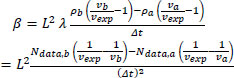
For two consecutive road parts {x1, x2} and {x2, x3} (or S1, S2), we define the parameter B, as the overall internal power of the road segments in Eq. (11):
 |
(11) |
Summing up, in this paper, we will use the highest 25% of B values, subject to βS1 < 0 & βS2 > 0. In further research, more assumptions can be tested to improve the accuracy of the prediction.
3. APPLICATION
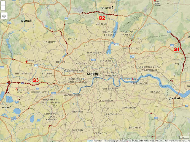
The relationships were applied using traffic flow data from the Highways England’s Application Programming Interface (API) [58] and car accident data from the Transport for London (TfL) API [59]. For both datasets, Rstudio was used to download data in JSON formats [60]. Highway cameras’ locations, together with car accidents, were inserted, projected, and plotted using their coordinates in Rstudio [61] and the “qtm” function for plotting [62]. As the car accidents dataset includes car accidents only from some areas of the highways, all cameras that do not intersect with these areas were excluded. The cameras left can be divided into three (3) groups: G1, G2, and G3 (Fig. 2).
Each of the three groups contains cameras capturing data from different directions. Only “A” and “B” cameras refer to the main road. The direction of “A” (“Away from London” or “clockwise”) cameras is opposite from “B” cameras (indicating “Back to London” or “anti-clockwise”) [63]. These cameras are going to be analyzed separately. This way, we have the following semi-groups: G1A and G1B, G2A and G2B, and G3A and G3B. The consecutive cameras were connected manually in ArcGIS with line segments. The characteristics of each camera were used to make it possible to understand which camera is first and which follows while driving. The line segments were then manually imported to Rstudio to use their lengths to calculate β and also to divide the car accidents into two groups (A and B). The car accidents closer to the left part of the road were considered to belong to the A group, and the car accidents closer to the right part of the road were considered to belong to the B group. This division was necessary because TfL does not give details regarding the direction of the cars in a convenient way.
| Cam\year | 2014 | 2015 | 2016 | 2017 |
|---|---|---|---|---|
| 1 | 8,711 | 28,219 | 31,868 | 31,588 |
| 2 | 8,735 | 28,266 | 31,868 | 31,588 |
| 3 | 8,711 | 28,242 | 31,868 | 31,588 |
| 4 | 8,711 | 28,266 | 31,868 | 31,588 |
| 5 | 8,735 | 28,218 | 31,868 | 31,588 |
| 6 | ... | ... | 31,868 | 31,588 |
| Site Name | Report Date | Time Period Ending | Time Interval | Average V (mph) | Total Volume |
|---|---|---|---|---|---|
| M25/5683A | 2016-01-01T00:00:00 | 0:14:00 | 0 | 71 | 79 |
| M25/5683A | 2016-01-01T00:00:00 | 0:29:00 | 1 | 70 | 41 |
| M25/5683A | 2016-01-01T00:00:00 | 0:44:00 | 2 | 69 | 102 |
| M25/5683A | 2016-01-01T00:00:00 | 0:59:00 | 3 | 70 | 173 |
The Highways England’s API was used to get each camera’s available traffic flow characteristics. To get the traffic data from the API, the ID of the camera was needed, as well as the target time period. Finally, all years except 2016 and 2017 were excluded from our analysis because some of the cameras were not operating during the whole year in all years, and these years were excluded because they could result in errors. For example, in the case of G1A, only in the years 2016 and 2017 we could find the same number of flow data for every camera (Table 1).
The matrices give basic information about the traffic and vehicle characteristics. Three (3) sets of information were kept: average speed, the volume of cars, and the date and time that the data were recorded. A sample of these characteristics is presented in Table 2.
Using these data, some transformations were necessary to calculate the internal power β parameter. These transformations can be found in the Appendix, along with information about the calculation of the expected velocities. This way, we could calculate the β parameter for each road segment (Table 3).
To apply the methodology proposed, we calculated the B values only for those consecutive road segments {xi, xi+2} with  , based on Eq. (10) (Table 4).
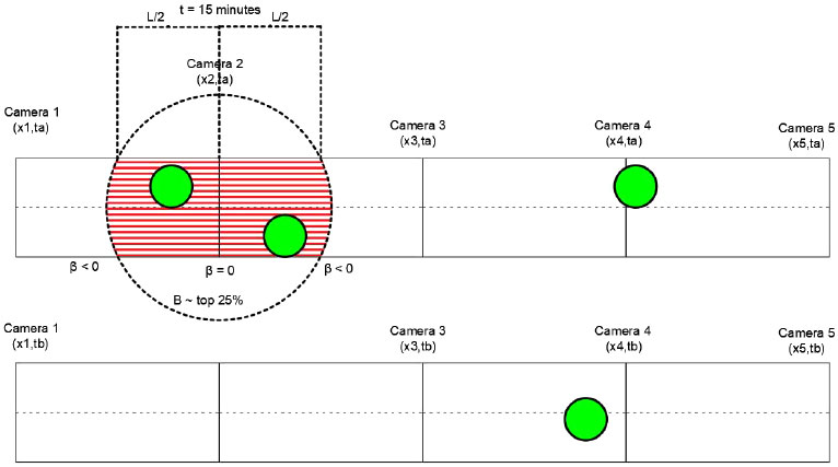
Finally, when these values appeared, we compared the number of car accidents in the road segments with the highest B values (top 25%) with the number of car accidents in all the other road segments (Fig. 3).
We expected to find car accidents in the examined areas. To test that assumption, we chose a smaller area inside the area {xi, xi+2} close to the middle camera xi+1. This area’s diameter was considered equal to L (the length of the road segments). We examined if a car accident occurred in that area (approximately 600 m) for a duration of 15 minutes. If an accident appeared under these circumstances, we would consider that accident to have been predicted. Finally, even though the methodology was applied to all six (6) groups: G1A, G1B, G2A, G2B, G3A, and G3B, the B areas were all excluded because they contained cameras that were not operating properly.
In Fig. (3), the accidents were represented using solid circles. If an accident occurred inside the circle, it was thought to have been predicted. In this specific case, using an area that is ¼ of the whole area and a time frame that is ½ of the whole time, we have predicted 50% of the car accidents. This means that a specific spatiotemporal section, which represents 1/8 of the overall, contains 50% of the car accidents (>> 1/8); therefore, the assumptions of this paper have been verified.
| - | Date & Time | L (m) | v (mph) | N (vehicles) | vexp (mph) | ∆t (sec) | βs |
|---|---|---|---|---|---|---|---|
| 1 | 1/1/2016 0:14 | 481 | 32.18 | 78 | 28.77 | 840 | -0.051 |
| 2 | 1/1/2016 0:29 | 481 | 31.73 | 40.5 | 28.77 | 900 | 0.047 |
| 3 | 1/1/2016 0:44 | 481 | 31.51 | 98 | 28.77 | 900 | 0.064 |
| 4 | 1/1/2016 0:59 | 481 | 31.51 | 172.5 | 28.77 | 900 | 0.058 |
| 5 | 1/1/2016 1:14 | 481 | 31.29 | 197 | 28.05 | 900 | 0.020 |
| Date & Time | B(x 0, x2) | B(x1, x3) | B(x2, x4) | B(x3, x5) |
|---|---|---|---|---|
| 1/1/2016 0:14 | - | 0.082 | - | - |
| 1/1/2016 0:29 | - | - | - | 0.019 |
| 1/1/2016 0:44 | - | - | - | - |
| 1/1/2016 0:59 | - | - | - | - |
| 1/1/2016 1:14 | - | - | - | - |
4. RESULTS AND DISCUSSION
The car accidents in the three areas examined during a period of two (2) years are 214. Based on data availability, the sum of the road segments examined in the areas G1A, G2A, and G3A is 77, each containing a camera in the middle. The available data for each camera corresponds to 63,456 15-minute entries. If these accidents were evenly distributed in space, then there would be 214/77=2.78 accidents in every road segment. Similarly, if the accidents were evenly distributed in time, there would be a probability of 2.78/63,456=4.3·10-5=0.0043% of having a car accident in every 15-minute entry. Equivalently, we get this percentile by diving the number of accidents by the time entries, multiplied by the number of cameras (spatial entries): 214/(63,456.77)=4.3·10-5 car accidents/ (approximately 600 m .15 minutes).
Nevertheless, car accidents are not evenly distributed in space and time. This paper shows that the areas with high B values correspond to a higher probability of car accidents. Using the highest 25% of B values of each road segment {xi, xi+2}, subject to 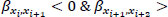 , we get 11 car accidents, which are considered as “predicted.” The condition applies to 249,420 spatiotemporal entries. We used the top 25% of them to search for car accidents around them, resulting in 62,355 spatiotemporal entries. Finally, the probability we get is 11/62,355=1.76·10-4=0.0176%, which is considerably higher than the previous one. This probability is lower in the area G1A and higher in G2A and G3A.
By dividing the probabilities, i.e., 1.76·10-4/4.3·10-5 = 4.09, we find that by using the proposed model, we can find four (4) times more car accidents compared to what we would have found if they were evenly distributed. As explained above, if we use lower time frames, this number will significantly increase; the lower the time frame, the more significant the increase and the same goes for real-time data.
Finally, we compared these results with the probability we get when we use 25% of the highest car volumes. The probability that we get is 2.14·10-5. This means that internal stress energy is a more effective indicator than high car volumes regarding car accident prediction.
The overall number of accidents (214) also includes accidents that have taken place in B parts because of inaccurate spatial exclusion. These accidents cannot be predicted using traffic data from the A parts. If the accidents in B areas were removed from the datasets, the probability of predicting a car accident would have been even higher than the even car accident distribution. We believe that the accuracy of a prediction can be radically improved in case more frequent data are available (e.g., every 2 minutes instead of 15 minutes).
CONCLUSION, PROPOSALS, AND ORIENTATIONS FOR FUTURE RESEARCH
In this paper, we propose a method that can be used to predict car accidents inspired by mechanics and the conservation of energy. The basic assumption is that drivers change their behavior during their trip to arrive on time at their destination. The drivers’ inability to fulfill their expectations during the trip is counted using an “internal stress energy” parameter. The more they feel they will be late, the more nervous they become, increasing their energy. Each driver behaves like an agent aiming for energy minimization. The model is applied in London Highways using traffic data from London Highways and car accidents data from TfL. Using two years’ data, we prove spatial variations of drivers’ internal stress “power” are connected with an increased probability of a car accident. More specifically, using the proposed model with 15-minute timeframes increased car accident prediction four (4) times compared to the evenly spatiotemporal car accident distribution. The model can be easily applied when live traffic data are available. With such data, we expect a dramatic improvement of the model as its accuracy increases and the time frame decreases. The proposed model can be tested in other areas to estimate its accuracy and potential uses. Overall, the model can be expanded to analyze real-time data to make predictions and help stakeholders act in dangerous conditions.
The novelty of this research is that it introduces the concept of “internal stress energy” and proves it to be a more effective car accident prediction indicator than high car volumes, given there are data of small timeframes or real-time data available. Nevertheless, the main limitation of the research is that the concept was tested in timeframes of not less than 15 minutes, a case in which even better results are expected.
In further research, the assumptions of the model can be studied. For example, it is interesting to find out if the traffic conditions become less dangerous when the drivers change their expectations and adapt to their environment. It is also interesting to find out if the probability of a car accident increases when the energy is radically released. Finally, neural networks can be used to find more accurate correlations between car accidents and the drivers’ internal stress energy, which might not be easily noticeable.
LIST OF ABBREVIATIONS
| API | = Application Programming Interface |
| ETSC | = European Transport Safety Council |
| EU | = European Union |
| TfL | = Transport for London |
AVAILABILITY OF DATA AND MATERIALS
The data that support the findings of this study were last accessed in December 10, 2023 on Highways England at http://trishighwaysengland.co.uk/detail/trafficflowdata, reference number: years 2016 and 2017, and on Transport for London at https://api.tfl.gov.uk/swagger/ui/index.html? url=/swagger/docs/v1%23!/AccidentStats/AccidentStats_Get#!/AccidentStats/AccidentStats_Get, reference number: years 2016 and 2017. These data were derived from the following resources available in the public domain: 1. Highways England: https://webtris.nationalhighways.co .uk/, and 2. Transport for London: https://api.tfl.gov.uk/.
The data processing results are available upon request by the corresponding author [D.N].
CONFLICT OF INTEREST
Dr. Dimitrios Nalmpantis is the Editorial Advisory Board Member for the journal The Open Transportation Journal.
APPENDIX
This part describes how the main equations are transformed to match the examined dataset. Traffic flow can be defined as the number of vehicles passing through a point for a period of time  . At the same time, flow is also the density of the cars in a road segment, multiplied by the average velocity of these cars Q = ρvλ. In this specific case, λ is used to indicate the number of lanes, as density is defined using the number of lanes. Finally, combining these two relationships, we get the density
  .
.
In these relationships, ∆t is predefined and depends on data availability. Assuming that the difference ∆t between ta and tb is the same as the time difference needed for the data “Ndata” to be collected, the relationship created in the methodology becomes Εq. (A.1):
 |
(A.1) |
Parameter β refers to a road segment {x1, x2}. Therefore, we get the values v and ρ using the following two cameras: the camera at the beginning of the road segment and the camera at the end. The average of the values of the two cameras is used to get the characteristics of the segment as shown in Eqs. (A.2 and A.3):
 |
(A.2) |
 |
(A.3) |
To better understand these relationships, the most important part is to remember that they refer to the same road segment for consecutive time periods (Fig. 4).
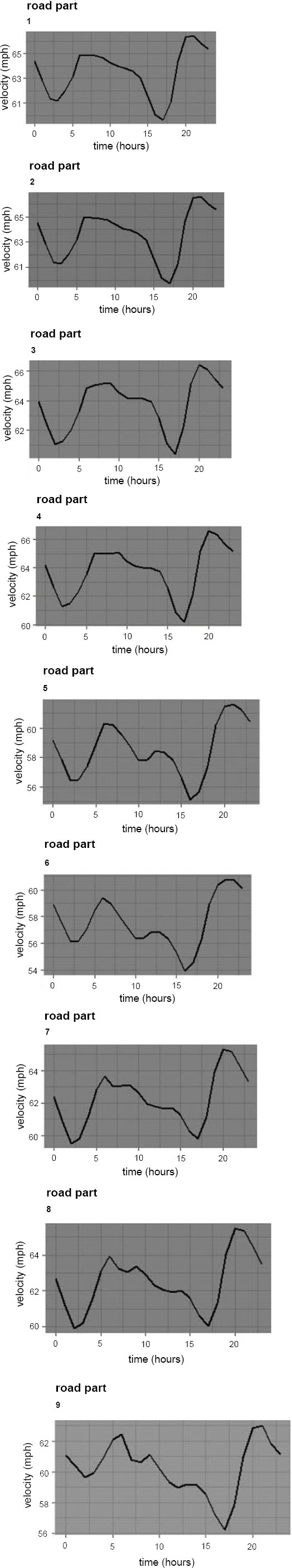
This way Na refers to the volume data recorded at ta and Nb refers to the volume data recorded at tb. The same applies to va and vb. ∆t is 15 minutes based on the API data availability. In any case, all N and v values are the result of getting the average values from the road segment’s starting and ending camera examined. Finally, vexp is the average hourly velocity of a specific road segment, calculated using average yearly values (Fig. 5) for an extended period of time. Drivers expect to find the road conditions they usually find at each road segment. We get these values using the 2-year data downloaded from the London Highways API.

