All published articles of this journal are available on ScienceDirect.

Forecasting Nighttime Frost-induced Black Ice Formation on Bridges Using Atmospheric Data
Abstract
Background
Faced with the tragedies caused by black ice in winter, especially on bridges, it is imperative to forecast black ice for preventive maintenance and to notify drivers approaching the dangerous spots.
Methods
In this study, three different machine learning algorithms-Deep Neural Network (DNN), Random Forest (RF), and Support Vector Machine (SVM)-were employed to predict nighttime black ice induced by frost on three bridges in Korea. Input data consisted of atmospheric data (air temperature, relative humidity, dew point, and differences between air temperature and relative humidity over two consecutive days) provided by the weather agency.
Results
To assess the employed models, reference data were generated based on the physical principle that ice forms when the pavement temperature is lower than the dew point temperature and negative. The pavement temperature was obtained using an infrared surface temperature sensor mounted on a maintenance patrol vehicle. Consequently, DNN and RF showed higher performance with an accuracy of 95%, followed by SVM with an accuracy of 92.5%.
Conclusion
Due to the use of easily obtainable atmospheric data, the findings of this study can be practically applied to preventive maintenance and driver information, thereby enhancing traffic safety.
1. INTRODUCTION
Many traffic accidents occur on wet and icy roads. A report indicates that in the United States, such conditions cause 1,705 deaths and 138,735 injuries annually [1]. According to a Swedish study, only 14% of drivers properly adjust their speed when navigating slippery surfaces [2]. Research from Portugal shows that the risk of an accident on icy roads is nine to ten times higher compared to dry roads [3]. Data from South Korea reveals that 122 fatalities resulted from 4,392 accidents on slick roads over five years. In 2019, a severe accident due to freezing rain on an icy road in South Korea caused seven deaths and numerous injuries; a similar incident occurred again in 2023 [4].
In Korea, all the tragic accidents that caused fatalities and garnered social attention have occurred on bridges at night. Bridges that transverse rivers or valleys tend to be affected by moisture or strong winds, indicating higher possibilities of black ice formation [5]. At night, drivers can hardly identify black ice on the road ahead. In the absence of precipitation, drivers normally regard their traveling routes as non-slippery. During winter nights, frost can induce black ice when traffic volume is low. Since drivers usually maintain high speeds on roads without precipitation, frost-induced nighttime black ice can cause severe accidents. In January 2024, frost-induced black ice caused a pile-up of 38 vehicles in Sejong City, Korea.
To addrress this issue, this study developed black ice forecasting models to improve the efficiency of anti-icing efforts, particularly for frost-caused black ice on bridges. Three widely recognized machine learning algorithms-Deep Neural Network (DNN), Random Forest (RF), and Support Vector, achine (SVM)-were explored to forecast black ice using atmospheric data (air temperature, relative humidity, dew point, and differences between air temperature and relative humidity over two consecutive days). With these forecasting models, nighttime black ice can be accurately predicted using readily available atmospheric data, enabling maintenance personnel to carry out anti-icing activities (such as patrolling and applying chemicals) and provide the predicted information to drivers approaching the hazardous location via variable message signs.
2. METHOD
2.1. Methods in Previous Studies
Black ice can form for various reasons [6], including freezing melted snow overnight, freezing rain on negatively tempered pavement, and frost bonding with the road surface. The first two causes can be predicted with atmospheric weather forecasting since they are caused by snow or rain. However, the last cause can only be detected through regular road maintenance patrols [7].
Physical models and regression analysis have primarily been used to predict black ice. Physical models use a surface energy balance principle based on heat conduction, convection, radiation, and vapor movement estimates to predict pavement temperature [8-11]. Regression models predict pavement temperature using different data, such as atmospheric data, geometry, and air temperature from probe cars [12-14]. However, both types of models have limitations. Physical models require hard data, such as pavement thickness, heat transfer rate of pavement material, and heat flux, which are not always obtainable, indicating that atmospheric data and pavement temperature alone cannot effectively forecast black ice. Regression models are relatively simple to understand but struggle with predicting variables that have a non-linear correlation.
To overcome the limitations of the previous methods, three machine learning models were used: DNN, RF, and SVM. The input data for these models consisted of readily available atmospheric data, which are provided by the weather agency on a real-time basis. This indicates that the suggested methodology can be practically applied in real-world practices without requiring substantial budget investments. Unlike conventional physical models that require various types of road weather data, the machine learning models developed in this study only necessitate easily accessible atmospheric data, thereby enhancing practicability. Additionally, machine learning models have been recognized for their superiority over conventional regression models. In summary, practicability and performance are the two primary advantages of the approach pursued in this study.
2.2. Prediction Method Explored in this Study
2.2.1. Deep Neural Network
A Deep Neural Network (DNN) is a type of machine learning algorithm that can analyze complex features from a given set of examples by utilizing multiple layers. Examples of popular deep learning categories include deep neural networks, recurrent neural networks, and convolutional neural networks, which have shown exceptional performance in various fields, including image processing, speech/audio recognition, and time-series data analysis, sometimes even surpassing human capabilities.
2.2.2. Random Forest
A Random Forest (RF) algorithm is a machine learning approach that consists of a group of decision trees, where each tree in the ensemble is built using a data sample drawn randomly and with replacement from a training set known as the bootstrap sample. To add more variety to the dataset and decrease correlation among decision trees, feature bagging is introduced as another source of randomness. The method for making predictions will depend on the problem being tackled; for a regression task, the individual decision trees are averaged, while for a classification task, the predicted class is determined by the most frequent categorical variable through a majority vote.
2.2.3. Support Vector Machine
A Support Vector Machine (SVM) is a type of supervised machine learning algorithm that is commonly utilized for classification and regression analysis. SVM models are typically considered non-stochastic binary linear classifiers, where instances are represented as points in a space domain and are mapped to separate groups based on the widest gap between them. New instances are then categorized by mapping them into the constructed space and placing them into one of the two categories based on the established gap function.
2.3. Baseline Data Generation for Evaluating Predicted Black Ice Information
In order to evaluate the accuracy of the predicted black ice information, baseline data is necessary. While using a reference device to measure road surface status would be the most reliable and straightforward method, it was not practical for this particular study due to the associated labor requirements, cost, and the need to acquire the device. Instead, a physical principle expressed in Eq. (1) was used, which states that frost on a pavement forms when the pavement temperature (Tp) is not only negative but also lower than the dew point temperature (Td).
 |
(1) |
The dew point temperature (Td) is the temperature at which air becomes saturated with moisture and water vapor begins to condense. The calculation of the dew point temperature is often done using the Magnus formula, which is a widely used method for this purpose [15]. Using the Magnus formula, the dew point temperature can be calculated from the actual vapor pressure (e) of the air. First, calculate the actual vapor pressure (e) using relative humidity (RH) and saturation vapor pressure (es(T)) using Eq. (2).
 |
(2) |
In Eq. (2), es(T) can be estimated using Eq. (3). In this context, T represents the air temperature in degrees Celsius (°C); a and b are empirically derived constants. Different sets of constants a and b are used depending on the temperature range and the type of surface (water or ice). For temperatures over liquid water, the typical values are 17.62 and 243.12°C for a and b, respectively.
 |
(3) |
Then, the dew point temperature (Td) can be calculated by rearranging the Magnus formula to solve for (Td) using Eq. (4). The dew point temperature computed by the Magnus formula is widely accepted due to its performance with an error of around 0.35°C [16].
 |
(4) |
To verify the Magnus formula, a wintertime highway segment was patrolled while measuring pavement temperature. The results showed that frost-induced black ice occurred (on the left) when the conditions for frost formation were met, whereas no black ice was observed (on the right) when those conditions were not met, as illustrated in Fig. (1). The patrolled roadway had a low traffic volume of fewer than 100 vehicles per hour [17].
3. RESULT
3.1. Data Collection
In this study, we equipped road maintenance vehicles with a road surface temperature sensor, as shown in Fig. (2). This sensor employs an infrared thermometer to measure the temperature of three specific bridges, which are designated as the 'black ice-prone segment' by the road agency. Nighttime maintenance patrols were conducted on these bridges on a daily basis during the winter. The sensor operates continuously while the vehicle is in motion, providing temperature measurements at intervals of 0.2 seconds. We collected pavement temperature data from three bridges (Fig. 3), each approximately 300 meters long, spanning from December 2021 to March 2023, encompassing two complete winter seasons. Data collection occurred over 397 days, with measurements taken once per day during nighttime hours. The sensor's precision is significantly improved by its narrow half-angle of 5°, ensuring accurate surface temperature readings [18]. When the temperature is 0°C, the sensor maintains an accuracy of ±0.3°C. Additionally, we obtained concurrent atmospheric data, including air temperature and relative humidity, from the nearest weather station operated by the weather agency during the same time period.
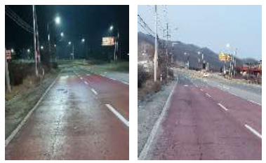
Pavement with frost (left) and without frost (right).
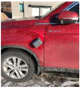
Surface temperature sensor.
3.2. Data Analytics
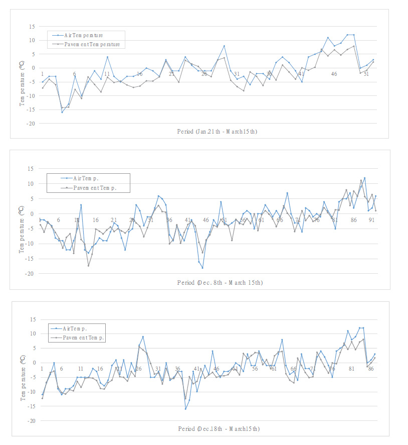
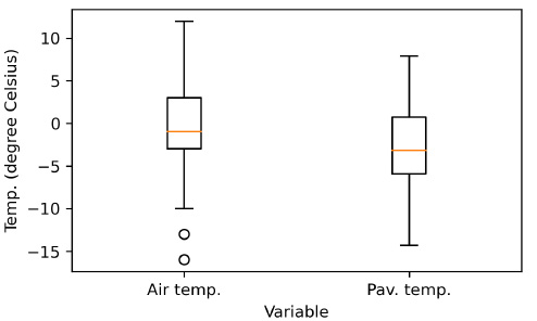
The pavement temperature data, collected at a sampling rate of 0.2 seconds, were aggregated to derive a single median value for each bridge. This median value serves as a representation of central tendency. Among the three common measures of central tendency (mean, median, and mode), the median is widely acknowledged for its resilience in mitigating the impact of extreme observations [19, 20]. Fig. (4) shows graphs of the pavement temperature and air temperature collected at the three bridges described above. The order of the graphs is the same as in Fig. (3). Overall, the bridge temperature was observed to be lower than the air temperature, and the variability was observed to be greater in the air temperature. As shown in Table 1, the average and maximum bridge temperatures were approximately 2°C and 4°C lower than the air temperatures, respectively. Conversely, the minimum air temperature was roughly 2°C lower than the bridge temperature. Unlike air temperature, which fluctuates significantly with airflow, pavement temperature is thought to exhibit relatively low variability due to the heat stored in the structure and the heat from passing vehicles.
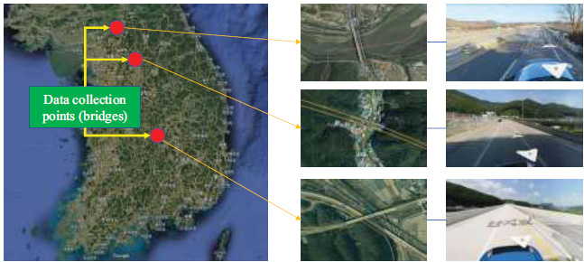
Data collection locations.
| Statistics | Air Tem. | Pav. (Bridge) Temp. |
|---|---|---|
| Mean | -0.30 | -2.47 |
| Standard deviation | 5.56 | 5.01 |
| Minimum | -16.00 | -14.30 |
| 25% | -3.00 | -5.93 |
| 50% | -1.00 | -3.15 |
| 75% | 3.00 | 0.73 |
| Maximum | 12.00 | 7.90 |
Air temperature vs. pavement (bridge) temperature.
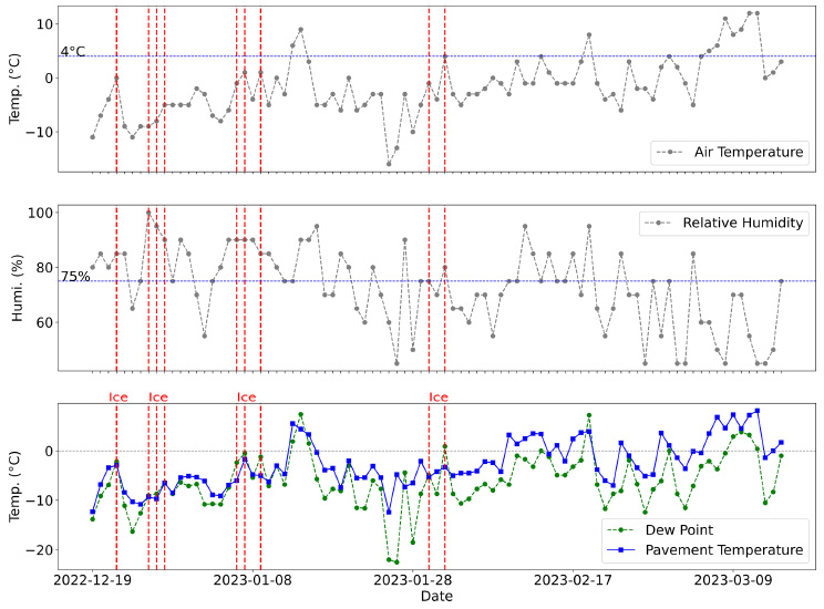
Fig. (5) illustrates the temperature and humidity characteristics observed in one of the three bridges during frost formation. The red dotted lines represent instances of frost formation as determined by equation (1), indicating when the pavement temperature falls below freezing and is lower than the dew point temperature. Upon examining the temperature and humidity patterns during frost formation, it becomes evident that, in most cases, the temperature rises after a sharp decline while humidity remains consistently above 75%. Furthermore, it is apparent that frost can occur even when the air temperature is above freezing, provided that the pavement temperature is below 0°C. The temperature difference between the air temperature and the bridge temperature was observed to be as much as 4°C. Based on the analysis conducted, it can be inferred that during winter, frost formation is more likely to occur when temperatures are on the rise, as long as the pavement temperature still remains below 0°C.
4. BLACK ICE PREDICTION
4.1. Building Blocks of Machine Learning Models
Based on the above-investigated results, we developed a nighttime black ice prediction model using atmospheric data. The input data for the machine learning models consisted of temperature, humidity, temperature difference from the previous and following days, humidity difference from the previous and following days, and dew point temperature, which were collected over a two-year period at the three points mentioned earlier. The baseline data were generated using equations (1-4) with the input data and pavement temperature data collected by patrol vehicles. We employed three well-known prediction models, namely DNN, RF, and SVM, which are known to have generally superior performance. Fig. (6) depicts the building blocks for the three models. Since the scale of each input data was different, we standardized the data using a standard scaler before training the models. The training and test sets were classified into a 7:3 ratio, and the dry/icing data ratios of the raw data were applied during classification to ensure a balanced distribution in both sets. The total data used for analysis consisted of 397 days, including 193 days of icy and 204 days of dry conditions.
Boxplot of air and pavement temperature.
Cases of frost-induced black ice formation.
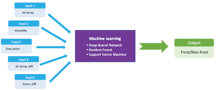
Building blocks of machine learning models.
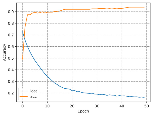
Learning process of deep neural network model.
4.2. Deep Neural Network
The DNN model was built using the TensorFlow Keras platform. As shown in Table 2, the model had a 30x20 hidden layer and a total of 821 parameters. The optimal number of hidden layers was determined with an error-and-trial process [21]. The rectified linear unit activation function was used, and the Adam optimizer was applied with 50 epochs. Fig. (7) shows the training process of the built model, using accuracy as the evaluation metric. As shown in Table 3, the predicted results of the model demonstrated overall satisfactory performance, with a particularly notable 100% prediction rate for icing conditions. Thus, the performance of the model was deemed satisfactory.
| Layer (type) | Output Shape | Number of Parameter |
|---|---|---|
| dense (Dense) | (None, 30) | 180 |
| dense_1 (Dense) | (None, 20) | 620 |
| dense_2 (Dense) | (None, 1) | 21 |
| Total params: 821 | ||
| Trainable params: 821 | ||
| Non-trainable params: 0 | ||
4.3. Random Forest
Random Forest is a prediction model that averages multiple decision trees, so it is crucial to determine the optimal number of decision trees. To achieve this while keeping other parameters fixed at constant values, decision trees ranging from 1 to 50 were investigated using accuracy as the evaluation metric. Consequently, the optimal number of decision trees was determined to be 11, as depicted in Fig. (8). Other parameters, excluding decision trees, were estimated using the “GridSearchCV” class from the sci-kit-learn library in Python. The resulting optimal parameters were determined to be {‘criterion’: entropy, ‘max_depth’: 10, 'max_features': auto, 'max_leaf_ nodes': 30, and 'n_estimators': 12}. Unlike other models, the RF model can calculate the importance of each input variable. Analyzing the widely used Gini-importance for impurity measurement, it can be seen from Table 4 and Figs. (9 and 10) that humidity and air temperature differences between consecutive days have the highest importance. As seen in Table 5, the performance of the model is also excellent.
| Classification | Prediction | ||
|---|---|---|---|
| Dry | Icy | ||
| Baseline | Dry | 0.919 | 0.081 |
| Icy | 0.000 | 1.000 | |
| Features | Humidity | Air Temp. Diff. | Dew point | Air Temp. | Humi. Diff. |
|---|---|---|---|---|---|
| Gini-Importance | 0.372 | 0.300 | 0.160 | 0.119 | 0.048 |
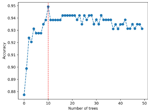
Searching process of the optimal number of trees.
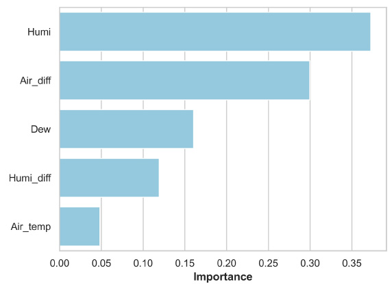
Feature importance for random forest model.
| Classification | Prediction | ||
|---|---|---|---|
| Dry | Icy | ||
| Baseline | Dry | 0.935 | 0.065 |
| Icy | 0.034 | 0.966 | |
| Classification | Prediction | ||
|---|---|---|---|
| Dry | Icy | ||
| Baseline | Dry | 0.887 | 0.113 |
| Icy | 0.034 | 0.966 | |
| Model | Accuracy | Precison | Recall | F1 Score |
|---|---|---|---|---|
| DNN | 0.950 | 0.906 | 1.000 | 0.951 |
| RF | 0.950 | 0.933 | 0.966 | 0.949 |
| SVM | 0.925 | 0.889 | 0.966 | 0.926 |
4.4. Support Vector Machine
Similar to the RF model, there are several parameters for model optimization in SVM as well. When training an SVM model, the performance of the model heavily depends on the parameter settings. The main parameters used in SVM are as follows:
4.4.1. Parameter C
C is a parameter that adjusts the penalty for misclassification in the SVM model. As C gets smaller, the model allows more misclassification, while as C gets larger, the model minimizes misclassification. If C is too large, the model may overfit, and if C is too small, the model may underfit.
4.4.2. Kernel
A function used to classify data nonlinearly in the SVM model. Commonly used functions include Linear, Polynomial, and Radial Basis Function (RBF).
4.4.3. Gamma
A crucial parameter when using the RBF kernel. As gamma gets smaller, the decision boundary widens, and as gamma gets larger, the decision boundary narrows. If gamma is too small, the model may underfit, and if gamma is too large, the model may overfit.
The optimal parameters were determined using the “GridSearchCV” class from the scikit-learn library in Python, and the resulting values were {'C': 100, 'gamma': 'auto,' and 'kernel': 'rbf'}. Table 6 shows the results predicted using the optimal parameters. Although the performance is somewhat lower than that of DNN and RF, the overall performance is satisfactory, with an accuracy of over 0.9.
5. DISCUSSION
Table 7 is a comparison table for three different models. Performance comparison was conductedusing accuracy, precision, recall, and F1 score, which, as expressed in Eqs. (5-8), are commonly used for evaluating machine learning models. DNN and RF showed the same performance overall, but in terms of the F1 score, DNN was the highest. Since the recall of DNN is 100%, there were no cases of predicting an icy surface as a dry surface, making it more satisfactory compared to other models.
 |
(5) |
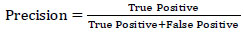 |
(6) |
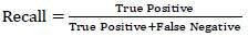 |
(7) |
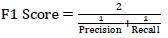 |
(8) |
It should be noted that the reference data employed in this evaluation is not the actual surface condition observed on the bridges but rather calculated values using road surface temperature and atmospheric data using widely-recognized physical principles. Even if the conditions for frost formation are met according to the physical principle, road icing may not occur in cases of high traffic volume [22] due to heat from the passing vehicles. Nevertheless, the results of this study can be highly regarded in the following perspectives. From the viewpoint of road administrators, if icing due to frost is expected, they should perform anti-icing activities (such as patrolling and applying anti-icing chemicals). In this regard, the results of this study can be usefully applied to real-world winter road maintenance activities and driver information systems.
CONCLUSION AND FUTURE STUDIES
Traffic accidents caused by black ice result in substantial social losses annually. In particular, frost-induced black ice forming on bridges during nighttime poses a significant threat to drivers due to its inherent difficulty in discernment. In this context, this study explored machine learning-based models for forecasting frost-induced black ice. Although the input data were readily available atmospheric data (air temperature, relative humidity, dew point, differences in air temperature, and relative humidity between two consecutive days), the prediction performances were satisfactory, with accuracies exceeding 90%. The forecast information was assessed using baseline data generated by a physical principle, with inputs being pavement temperature data obtained using an infrared surface temperature sensor mounted on a maintenance patrol vehicle. The main findings of the application of the three machine learning models are as follows:
- The DNN model achieved the highest F1 score of 0.951.
- The RF model obtained the second-highest F1 score of 0.949 with an optimal number of 11 trees.
- The SVM model demonstrated the lowest F1 score of 0.926 among the three models.
- The hyperparameters of the RF and SVM models were automatically optimized using the “GridSearchCV” class from the sci-kit-learn library in Python.
- Relative humidity and the difference in air temperature between two consecutive days were found to be highly important for black ice forecasting in the RF model.
Analyses were performed to investigate the characteristic of bridge pavement temperature. As a result, the average bridge temperature was approximately 2°C lower than the air temperature. Also, bridge temperature exhibited relatively lower variability compared to air temperature, possibly due to the latent heat of the concrete structure and heat from passing vehicles. Furthermore, frost-caused black ice develops only when the air temperature is lower than 4°C and relative humidity is higher than 75%. Interestingly, frost-induced black ice is more likely to form when the temperature is rising rather than falling under subzero temperature conditions.
Conventionally, black ice information can be obtained using expensive road weather sensors. While installing these sensors is considered the best option, budget constraints often prevent road managers from acquiring black ice information. In this regard, this study is notable because it demonstrates that black ice information can be obtained without installing road weather sensors, using readily available atmospheric data provided by the weather agency. However, the machine learning models created in this study were evaluated solely based on baseline data derived from a physical principle. In the future, if feasible, baseline data should be gathered from field observations using road weather sensors that accurately measure road slipperiness to obtain a more reliable result.
AUTHORS’ CONTRIBUTION
The author confirms sole responsibility for the study’s conception and design, data collection, analysis and interpretation of results, and manuscript preparation.

