All published articles of this journal are available on ScienceDirect.

Estimation of Trip-based Generation Models and Calibration of Mode Choice Models for the American Travel Behavior
Abstract
Background
The National Household Travel Survey (NHTS) is the primary national dataset for analyzing personal and household travel trends. It covers daily non-commercial travel across all modes and details information on travelers, their households, and their vehicles.
Materials and Methods
The NHTS includes critical data for calibrating travel demand models, such as vehicle details (number and type), individual demographic characteristics (age, gender, employment), and household demographics (income, ownership status, size, race). In this study, we utilized the 2017 NHTS summary statistics to estimate individual trip generation models, differentiating between weekdays and weekends. By comparing factors influencing daily person trips during these periods, we aimed to discern distinctions between the two models. Additionally, we calibrated a mode choice model to understand the impact of trip purpose, duration, household income, and the ratio of available vehicles to household size on the chosen mode. Our analysis focused on identifying and quantifying the factors influencing travel behavior, providing insights into how various variables affect the number of trips and mode choices.
Results
The results indicated variations between weekday and weekend models, with the presence of non-workers and individuals' education levels emerging as crucial factors for weekday travel. Conversely, the existence of children, household income level, and personal yearly miles driven were identified as significant factors affecting weekend travel. Additionally, common characteristics such as household size and urban residence were substantial in both models. The Multinomial regression analysis investigated the correlations between individual, household, activity, and trip characteristics and the modes of transportation selected by travelers. The most significant factors influencing an individual's mode choice are household income, the ratio of available vehicles to household size, and activity purpose.
Discussion
The study compared weekday and weekend travel behavior using trip-based generation models. Weekday travel was significantly influenced by non-workers and education levels, while weekend travel was more affected by factors like the presence of children, household income, and annual kilometers traveled. Both models emphasized the role of household size and urban residence in shaping travel patterns. The research also examined transportation mode choice, with validation confirming the high accuracy and robustness of the mode choice model in predicting travel behavior.
Conclusions
The study findings are valuable to transportation planners, policymakers, and urban mobility experts aiming to enhance the efficiency and effectiveness of transportation systems. By offering a detailed understanding of individual and household travel patterns, the research enables data-driven interventions that support policy decisions, such as optimizing transit routes, enhancing infrastructure for active transportation, and managing congestion.
1. INTRODUCTION
The travel forecasting process occupies a central role in urban transportation planning. Travel forecasting models, which are essential for projecting future traffic, provide the foundation for evaluating and determining new road capacities, transit service changes, and modi- fications in land use policies and patterns. In travel demand modeling, human travel behavior is attempted to be simulated through a series of mathematical models [1]. These models are developed through a sequential process that addresses questions related to traveler decisions. These steps include trip generation, trip distribution, mode choice, and route assignment [2].
Travel forecasting models play a crucial role in promoting sustainable urban transportation systems. They help urban planners and policymakers understand potential future scenarios by providing insights into how changes in infrastructure, transit options, and land use might influence travel behavior [3]. By simulating various scenarios, these models allow for more informed decision-making, enabling the design of transportation systems that better meet the needs of the population while considering environmental and economic factors. The comprehensive nature of travel demand modeling ensures that a wide range of variables and their interdependencies are considered, making it an essential tool in the planning and development of sustainable urban transportation systems [4].
The four-step model is the primary tool for forecasting a transportation system's future demand and performance. The road traffic estimation or transportation demand models are essential to planning [5]. Planners must comprehend and execute transportation demand or traffic estimation models before initiating any planning and evaluation of roads or other transportation initiatives [6]. Effective traffic forecasting is crucial for ensuring the success of the planning process. According to Chatzis’s study [7], anticipating transportation demand and road traffic for metropolitan areas to assist in transportation planning began in the mid-1950s. This underscores that numerous transportation demand models have been developed since then. Despite significant advancements in this field, traffic forecasting remains an area that continues to evolve and expand. Researchers have invested considerable time and resources in developing transport demand forecasting models tailored to specific regions or countries. Meanwhile, practitioners consistently strive to choose the most suitable model for application in their study areas [7, 8].
Inaccurate predictions of transportation demand can lead to inaccurate decisions, potentially causing signi- ficant economic and social impacts, especially in large-scale projects [9]. Aldian emphasized that inaccurate estimations often incur higher costs in developing countries, mainly because a substantial portion of their projects is typically financed through foreign organizations [10]. The primary objective of developing travel demand modeling is to ensure a close correspondence between forecasted values and real-world outcomes [11]. This objective depends on the appropriateness of the model structure, the accuracy of the data, and the confidence level associated with the forecasting values of variables [11]. Tailoring a model optimally suited for a specific area is increasingly crucial in transport planning [12]. Various issues, such as congestion and air quality degradation, are generally linked to travel and are specifically associated with an increase in people's travel time, a rise in vehicle miles traveled, and changes in household and personal structures [12].
Further, the accuracy of transportation demand fore- casting directly impacts infrastructure planning, invest- ment decisions, and policy formulation. Incorrect demand predictions can lead to underutilization or overutilization of resources, misallocation of funding, and long-term economic inefficiencies [6]. For instance, overestimating transportation demand may result in unnecessary expan- sions, leading to wasted financial resources and potential environmental degradation. This potential for environ- mental degradation should be a cause for caution. Con- versely, underestimating demand could cause congestion, increased travel times, and a deterioration in the quality of life for commuters [6].
Furthermore, the methodological robustness of travel demand models is crucial for their reliability [13]. These models can enhance their predictive power by incor- porating diverse variables, such as demographic changes, economic trends, and technological advancements. However, continuous validation and calibration against real-world data are essential to ensure their accuracy over time. This process is key to maintaining the reliability of travel demand forecasts and should be a priority for all involved in transportation planning [14]. Thus, accurate transportation demand predictions are vital for effective transport planning and sustainable development. They require a multifaceted approach involving rigorous data analysis, appropriate model selection, and ongoing refinement. Addressing these challenges empowers policy- makers to make informed decisions that promote economic growth, social well-being, and environmental sustainability [6].
The exploration of weekday travel has received considerable attention in numerous research studies compared to investigations into weekend travel [15]. Given that a significant portion of weekday travel occurs during peak morning and evening hours, which are associated with congestion, there is a need for increased focus in this area. Conversely, congestion has been notably observed in most major cities worldwide during weekends [16]. Furthermore, weekend travel distinctly differs from weekday travel in various aspects, including variations in the distance range between origins and destinations, primary purposes, modes of transportation, and shifts in peak times [17]. Understanding the demand for weekend travel is essential for real-time traffic operation and management [18]. Therefore, comprehending both weekend and weekday travel demands for improved planning and operations.
This research offers a novel approach to understanding the dynamic differences between weekday and weekend travel patterns by generating individual trip-based models. Unlike traditional studies, which primarily focus on aggregate trends e.g., [19, 20], this work delves into the granular, individualized variations that emerge due to socioeconomic, spatial, and temporal constraints. This study also considers contemporary influences such as technological advancements, societal shifts like the rise of 24-hour services, and demographic changes such as immigration, all of which add complexity and unpredict- ability to modern travel behavior. This comprehensive analysis extends beyond conventional trip-generation models, providing a deeper understanding of how and why travel behavior shifts throughout the week.
This research's novelty lies in its detailed examination of individualized travel patterns and its exploration of how these patterns respond to predictable and unpredictable societal factors. This study bridges a significant gap in current transportation research by addressing the underexplored variations in travel behavior across different days of the week, offering insights that are crucial for developing adaptive and resilient urban transportation networks. The findings are expected to inform more targeted and effective traffic management, public transportation planning, and urban mobility strategies tailored to the specific demands of both weekday and weekend travel.
Moreover, the second innovative contribution of this research lies in developing mode choice models that estimate travel preferences across various transportation modes, including private vehicles, public transit, walking, and bicycling. Unlike standard mode choice models, which often treat travel modes as static preferences, this study emphasizes the dynamic nature of mode selection, linking it to the variations in travel patterns observed throughout the week. By doing so, the research provides a more nuanced understanding of mode choice that can better inform transportation investments, policy decisions, and long-term urban planning. This methodological approach highlights the complexity of modern travel behavior and offers valuable insights into the design of sustainable and efficient transportation systems.
2. SCOPE AND STUDY OBJECTIVES
The primary objective of this innovative study is to understand the variations in travel patterns between weekday and weekend trips, utilizing individual-level characteristics in trip-based generation models. Achieving this goal involves conducting a Negative Binomial (NB) regression analysis. Consequently, we aim to identify and investigate the factors influencing household trips per day on weekdays and weekends, comparing these factors in a novel way that has not been explored before.
The second objective is to estimate a model for travel modes based on the number of trips completed by each mode. This involves employing Multinomial Logistic (MNL) regression models. Specifically, we aim to discern the impact of trip purpose, trip duration, household income, and household size ratio to available vehicles on the chosen mode. These estimates are expected to provide valuable insights for transportation planning and decision-making.
3. DATA
The data utilized in this study is sourced from the National Household Travel Survey (NHTS) website [21], which provides summary statistics for demographic characteristics and travel activities conducted in 2017 by the Federal Highway Administration (FHWA). This dataset presents valuable opportunities for examining weekday and weekend travel behaviors and is an excellent resource for future policy analyses. The dataset encompasses detailed information on individuals' demographics and socioeconomic characteristics, including employment status, income, gender, age, and education level. Additionally, it includes household information such as size, income, ownership status, and race, as well as vehicle and trip-specific details, including license status, trip durations, and origin-destination times. It is crucial to emphasize that the data exclusively documents daily non-commercial travel by any mode of transportation.
3.1. Individual Trip-based Generation Models Data
In this study, trip generation models were estimated at an individual level. However, certain crucial variables at the household level, such as household size and the number of vehicles per household, were deemed essential. Excel tools and functions, including Pivot Table, VLOOKUP, AVERAGEIFS, MINIFS, and MAXIFS, were employed to facilitate the merging and definition of these variables. The filter tool was also utilized to eliminate unnecessary data entries, such as responses like 'I don't know' or 'prefer not to answer'. Furthermore, logical operations were applied to exclude certain variables, such as the 'availability of computers in the home' and 'frequency of internet usage', from the analysis.
Prior to analysis, the data underwent comprehensive preliminary cleaning procedures. Weekday records were separated from weekend records, and certain individuals were excluded from the original sample. For instance, households with significant inconsistencies, such as a discrepancy between the number of cars and the number of drivers (e.g., number of cars = 7 and number of drivers = 0), were excluded from the analysis. Outliers were systematically removed from the dataset. As a result, 34,485 individual observations were selected for the weekend regression analysis, while 119,785 individual observations were used for the weekday regression analysis.
3.2. Mode Choice Model Data
The dataset used to estimate the mode choice model was derived from the trip-level database. A total of 976,744 trip observations underwent filtering and cleaning processes to calibrate the MNL functions for each mode choice. Of these, 819,610 trip observations —approximately 90% of the total—were utilized for estimating the mode choice model, while the remaining observations were allocated for forecasting and validation purposes.
The independent variables in our MNL model included factors related to the alternatives, describing individual characteristics (such as household income and the ratio of available vehicles to household size) and trip character- istics (such as trip purpose and trip duration). Trip purpose and household income variables were categorized into five distinct groups, while trip duration and the ratio of available vehicles to household size were treated as continuous variables.
4. METHODS
4.1. Individual Trip-based Generation Models
NB regression is the same as conventional multiple regression, except that the dependent variable (Y) is an observed count that follows the NB distribution. As a result, the potential values of Y are the non-negative integers 0, 1, 2, 3, and so forth.
In trip-generation studies, the NB regression analysis is a valuable tool for developing prediction functions that estimate the trips generated by individuals or households [22]. This regression model is designed to establish a relationship between the explanatory variables and the dependent variable using an exponential equation. The standard form of the NB regression equation model is as follows:
 |
Where:
Y is the dependent variable (count of number of person trips). X1, X2 and Xn are independent variables (e.g., household size, number of cars, income, etc.) β1, β2 and βn are regression coefficients representing how much y changes, and
4.2. Mode Choice Model
4.2.1. The Utility Theory's Fundamental Structure
The utility is the determining factor in an individual's mode preference [24]. This factor is typically derived from the attributes of alternatives. Using the utility maxi- mization rule, an individual chooses an alternative from the options that maximize their utility. In the individual's choice set, the utility function (U) is defined as selecting an alternative if its utility exceeds that of all other options. This can be expressed as an alternative (i) that is chosen from a set of different options (j) on the condition that the utility of alternative (i) is either equal to or greater than the utility of all options (j) in the choice set (C). The utility function of a mode choice by a traveler (i) from other mode options (j) is represented by (Ui).
 |
Where:
Uin: is the utility function of the alternative (i) to the traveler (n),
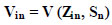
Vin: is the analyst's estimation of the observable or deterministic portion of the utility, and
εin: is the error or the portion of the utility that is unknown to the analyst.
The goal of mode choice modeling is to evaluate the traveler's behavior to determine the mode choice that will optimize utility among the available alternatives.
4.2.2. The Utility of Alternatives Selected by Travelers
The deterministic utility component comprises the variables associated with the mode choice alternatives that the traveler selects, describing the individual and trip characteristics. Non-motorized, private, public, and taxi travel comprise the other options examined in this investi- gation. The utility function that is generally deterministic is as follows:
 |
Where:
Zin: is the alternative-specific Attributes
Sn: is the socioeconomic characteristics.
And it can be represented as follows:
 |
Where:
Vin: is the utility value of mode choice (i) by traveler (n),
Xik: is the mode choice (i) by traveler (n), which includes non-motorized, Private car choice, public transport, and taxi,
β: is the intercept coefficient, and
β 1,2,…k: is the coefficient of the independent variable/s associated with the alternatives characterizes individual and trip features, which are included in our study: trip duration, activity purpose, individual income, and the ratio of the available vehicles to household size.
4.2.3. The Multinomial and Nested Logit Models
Random utility theory provides a concise explanation of the mode choice process. This study implements MNL analyses to examine and identify the influence of variables associated with travelers and mode alternatives on mode choices. The coefficients of the fundamental model are also estimated in the analysis.
In the context of travel behavior analysis, the utility function technique is employed to ascertain the mode choice. MNL is widely acknowledged as one of the most effective models for modeling mode choices. Mode choice models establish statistical relationships between the attributes of the available alternatives and the choices made by individual travelers. In the MNL model, it is presumed that the components of the utilities for the various sets of other options are independent. MNL expresses the relationship between the dependent and independent variables in terms of utility.
The Nested Logit (NL) model organizes alternatives into hierarchical groups, while the MNL model treats all alternatives equally. In practice, MNL models are more commonly used than NL models within the utility maximization framework because the MNL model allows for the estimation of choice probabilities based on the characteristics of both the travel modes and the travelers. To assess the validity of the MNL model’s assumption of Independence from Irrelevant Alternatives (IIA), the Hausman & McFadden test will be applied in this study. If the IIA assumption is violated, an NL model will be calibrated to account for the structure of nested alternatives.
5. RESULTS AND DISCUSSION
5.1. Trip Generation Models
The estimation process necessitates a file comprising one record for each surveyed individual. An individual record example may encompass continuous, dummy, or indicator variables such as Workers count per Household, Number of adults per Household, Yearly miles personally driven, and Number of drivers per Household as a Continuous Variable (CV). Additionally, variables like the existence of children within the Household, Gender (Male), Household in an urban area, and House ownership as a Dummy Variable (DV) are included. Income level, Household size, Number of vehicles per Household, Respondent age, and Respondent education level are Indicator Variables (IV).
5.1.1. List of Variables
This section delineates the variables assessed while estimating individual trip-based generation models, as illustrated in Table 1.
| List of Variables | Description |
|---|---|
| CNTTDTR | Number of trips per individual |
| YEARMILE | yearly miles personally driven |
| NUMADLT | number of adults per household |
| DRVRCNT | number of drivers per household |
| WRKCOUNT | Number of workers per household |
| homown | If home Own=1, otherwise=0 |
| Male | If gender is male=1, otherwise=0 |
| children | If children exist in a household =1, no children=0 |
| urban | Household in an urbanized area=1, otherwise=0 |
| inc | Household income of the respondent: 1= <$15000 (poverty level) 2= $15000-$50000 (low income) 3= $50000-$100000 (middle income) 4= $100000-$150000 (upper middle income) 5= >$150000 (high income) |
| vehcount | Number of available household vehicles: 0= zero vehicles/hh 1= one vehicle/hh 2= two vehicle/hh 3= three vehicle/hh 4= 4+ vehicle/hh |
| Hhsize | Household size of the respondent: 1= one person 2= two individuals 3=3 individuals 4= 4+ individuals |
| rage | Respondent age: 1=11-18 years old 2= 18-50 years old 3= >50 years old |
| highedu | Respondent education level: 0= less than high school 1= high school graduate or GED 2= college, Bachelor's, graduate, or professional degree |
| Nonworker | if a non-worker individual =1, otherwise=0. |
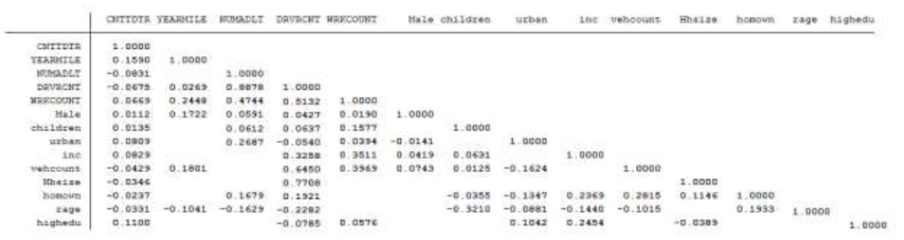
Spearman correlation test for the weekends individual trip-based generation model.
NOTE: Blanks mean no significant correlation.
5.1.2. Weekends Generation Model
The estimation of the NB regression model has typically been carried out using limited information. This approach initially involves estimating the correlation of parameters through a suitable correlation test, depending on the type of data under consideration. This study conducted a Spearman correlation test to assess the correlations among all variables, as illustrated in Fig. (1).
The Spearman correlation coefficient is calculated using ranked variables and assesses the strength and direction of the association between two variables. Unlike the Pearson correlation, which measures linear relationships between continuous variables, Spearman's coefficient is suitable for ordinal variables, whether they are continuous or discrete. Given that our data encompass three types of variables (CV, IV, and DV), a Spearman correlation test is more appropriate than a Pearson correlation test. The correlation results matrix is presented in Fig. (1) below and was generated using STATA software [23].
5.1.2.1. Parameter Estimates
The coefficients reflect the relationships between the explanatory variables and the person trip, while the count of individual trips is the outcome measure of the estimated model. Under the assumption that the number of trips has a natural ordering from zero to the maximal number of trips, the response variable (trips) is ordinal. The Pseudo-R2 value quantifies the extent to which the model accurately forecasts the data compared to the absence of any action. The interpretation of this statistic should be approached with caution, as it is frequently a minor value. Table 2 displays all parameter estimates for the subsequent person trip-based NB regression models; two models were predicted.
1) Y = f (Hhsize, urban, YEARMILE, children, inc).
2) Y = f (Hhsize, rage, WRKCOUNT, Male).
Given that the Pseudo-R2 value for Model 1 is marginally more significant than that of Model 2, it can be inferred that Model 1 exhibits a higher level of efficacy in predicting the data.
Incidence Rate Ratio (IRR) represents the estimated rate ratio for a one-unit increase in the math standardized test score while holding the other variables constant in the model. This ratio aids in the interpretation process of the models. Table 3 presents the IRR results for the weekend person trip-based generation model (Model 1).
5.1.3. Weekdays Generation Model
A new dummy variable, 'Non-worker’, was introduced into the dataset, assigned a value of 1 if an individual is a non-worker and 0 otherwise. Subsequently, a Spearman correlation test was performed using STATA software [23], as shown in Fig. (2).
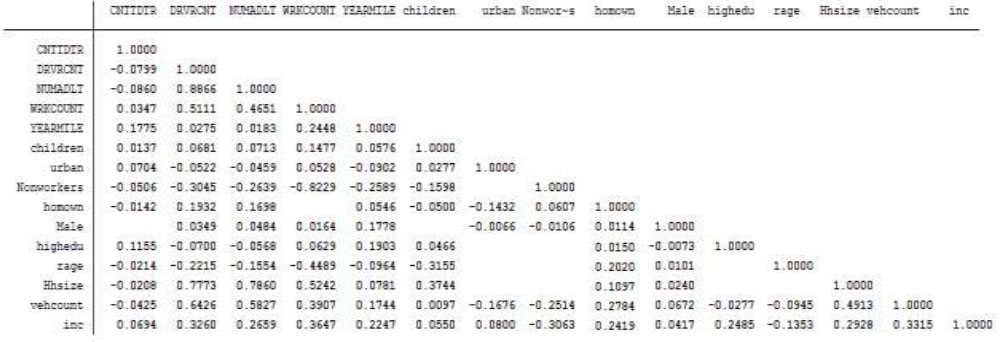
Spearman correlation test for the weekdays individual trip-based generation model.
Note: Blanks mean no significant correlation.
| Parameter Estimates | ||||||
|---|---|---|---|---|---|---|
| Weekends Model 1 | Weekends Model 2 | |||||
| Coeff. | Z-test | P-value | Coeff. | Z-test | P-value | |
| Constant | 0.985 | 40.42 | 0.000 | 1.095 | 30.16 | <0.00 |
| Household size 2 | -0.118 | -9.10 | 0.000 | -0.110 | -8.60 | <0.00 |
| Household size 3 | -0.191 | -11.52 | 0.000 | -0.221 | -12.78 | <0.00 |
| Household size 4 | -0.166 | -10.00 | 0.000 | -0.218 | -12.27 | <0.00 |
| Income 2 | 0.072 | 3.08 | 0.000 | --- | --- | --- |
| Income 3 | 0.171 | 7.37 | 0.000 | --- | --- | --- |
| Income 4 | 0.222 | 9.14 | 0.000 | --- | --- | --- |
| Income 5 | 0.240 | 9.66 | 0.000 | --- | --- | --- |
| Urban | 0.147 | 13.42 | 0.000 | --- | --- | --- |
| Yearly-Miles-driven | 0.000007 | 16.69 | 0.000 | --- | --- | --- |
| Children | 0.060 | 3.26 | 0.001 | --- | --- | --- |
| Respondent-age 2 | --- | --- | --- | 0.209 | 6.16 | <0.00 |
| Respondent-age 3 | --- | --- | --- | 0.136 | 3.92 | <0.00 |
| Workers count | --- | --- | --- | 0.078 | 13.50 | <0.00 |
| Male | --- | --- | --- | 0.019 | 2.08 | <0.00 |
| Pseudo-R2 value | 0.6341 | 0.5972 | ||||
| Weekends Model | |||
|---|---|---|---|
| IRR | Z-test | P-value | |
| Constant | 2.679 | 40.42 | <0.00 |
| Household size 2 | 0.888 | -9.10 | <0.00 |
| Household size 3 | 0.826 | -11.52 | <0.00 |
| Household size 4 | 0.847 | -10.00 | <0.00 |
| Income 2 | 1.075 | 3.08 | <0.00 |
| Income 3 | 1.187 | 7.37 | <0.00 |
| Income 4 | 1.249 | 9.14 | <0.00 |
| Income 5 | 1.271 | 9.66 | <0.00 |
| Urban | 1.158 | 13.42 | <0.00 |
| Yearly-Miles-driven | 1.000007 | 16.69 | <0.00 |
| Children | 1.062 | 3.26 | 0.001 |
| Pseudo-R2 value | 0.6341 | ||
| Parameter Estimates | |||
|---|---|---|---|
| Weekdays Model | |||
| Coeff. | Z-test | P-value | |
| Constant | 1.171 | 88.30 | <0.00 |
| Household size 2 | -0.098 | -17.11 | <0.00 |
| Household size 3 | -0.113 | -14.89 | <0.00 |
| Household size 4 | -0.049 | -6.73 | <0.00 |
| Education level 1 | 0.082 | 6.53 | <0.00 |
| Education level 2 | 0.250 | 21.40 | <0.00 |
| Non-Worker | -0.073 | -14.33 | <0.00 |
| Urban | 0.085 | 17.02 | <0.00 |
| Pseudo-R2 value | 0.5382 | ||
| Weekdays Model | |||
|---|---|---|---|
| IRR | Z-test | P-value | |
| Constant | 3.226 | 88.30 | <0.00 |
| Household size 2 | 0.906 | -17.11 | <0.00 |
| Household size 3 | 0.893 | -14.89 | <0.00 |
| Household size 4 | 0.952 | -6.73 | <0.00 |
| Education level 1 | 1.085 | 6.53 | <0.00 |
| Education level 2 | 1.284 | 21.40 | <0.00 |
| Non-Worker | 0.930 | -14.33 | <0.00 |
| Urban | 1.089 | 17.02 | <0.00 |
| Pseudo-R2 value | 0.5382 | ||
5.1.3.1. Parameter Estimates
The model was iteratively refined, and the predicted results are presented below. Table 4 displays the final iteration coefficient results for the weekday person trip-based regression model. Two iterations were conducted, with the “rage” variable deemed insignificant in the first iteration.
Iteration 1: Y = f (highedu, Hhsize, Nonworkers, rage, and urban).
Iteration 2: Y = f (highedu, Hhsize, Nonworkers, and urban).
 |
5.1.4. Interpretation of the Regression Models Results
1). Final Weekends Generation Model
Individual trips (Y) = EXP (0.9854 + 0.1471 Urban + 0.000007 Yearly-miles + 0.0604 children – 0.1183 (HHsize=2) – 1.91 (HHsize=3) – 1.66 (HHsize=4) + 0.072 (income=2) + 0.1714 (income=3) + 0.222 (income=4) + 0.2397 (income=5).
2). Final Weekdays Generation Model:
Individual trips (Y) = EXP (1.171 + 0.082 (education level = 1) + 0.25 (education level=2) – 0.098 (HHsize=2) – 0.1126 (HHsize=3) – 0.049 (HHsize=4) – 0.0726 (Non-workers indicator) + 0.085 urban.
For the weekend model, a unit increase in yearly miles driven personally results in a marginal 0.0007% increase in individual trips, indicating a relatively small impact. Additionally, the presence of indicator variables (urban, children, and income levels 2, 3, 4, 5) is associated with an increase in the number of person trips by (15.8%, 6.2%, 7.5%, 18.7%, 24.9%, and 27%), respectively. Conversely, the presence of the indicator variables for household sizes 2, 3, and 4 leads to a decrease in the number of person trips generated by (11.2%, 17.37%, and 15.3%), respectively. Alternatively, the results can be interpreted using the NB coefficient values, which indicate their impact on the log odds of the dependent variable and the number of person trips generated. For instance, the log odds of person trips increased by 0.06 if a household contains children.
Our findings not only provide valuable insights but also validate our initial expectations. We anticipated a direct proportional relationship between the number of weekend trips generated by an individual and income level, and an inverse proportional relationship with household size. These expectations were indeed met. Additionally, the presence of children in a household was expected to contribute more significantly to an increase in generated trips during weekends compared to weekdays, and our research confirmed this. Furthermore, we hypothesized that urbanized areas would have a more pronounced impact on the number of individual trips generated compared to rural areas, and our findings align with this hypothesis.
Similarly, in the weekday model, indicator variables (urban and education levels 1, 2) are associated with an increase in the number of person trips by (8.9%, 8.5%, and 2.8%), respectively. Additionally, the presence of the indicator variables (household sizes 2, 3, 4, and Non-workers) decreases the number of person trips generated by (9.4%, 10.7%, 4.8%, and 7%), respectively.
When comparing the factors affecting both models, it becomes evident that household size and the type of area (urban vs. rural) have nearly identical effects on travel behavior across weekdays and weekends. However, a critical distinction arises with non-workers, who contribute to a decrease in work-related trips, particularly on weekdays, when commuting for work is a major component of travel. However, the most significant and unexpected finding is the strong influence of education level on the number of weekday trips. Specifically, individuals with lower education levels tend to make more trips. This highlights a critical insight: education has a substantial impact on trip generation, with those having lower educational attainment potentially engaging in more frequent travel, which is essential for understanding broader patterns in weekday mobility. This point emphasizes the importance of considering education as a pivotal factor in travel behavior analysis.
5.2. Mode Choice Models
5.2.1. List of Variables
This section delineates the variables considered when estimating the mode choice model, as illustrated in Table 6.
5.2.2. Alternative-specific Mode Choice Model
In this model specification, the coefficients of the explanatory variables were presumed to be alternative-specific, indicating variations across the different alter- natives. Subsequently, an MNL model will be employed for socioeconomic variables (household income and ratio of available vehicles to household size) and alternative-specific attributes (trip purpose and duration).
Fig. (3) presents the results of the Spearman correlation test conducted using STATA software [23] for all variables included in the mode choice model. A notable correlation is evident between the transport mode (dependent variable) and the other explanatory (independent) variables, while an insignificant correlation was found among the independent variables.
| Variable | Description |
|---|---|
| mode |
Trip mode chosen:
0 = Non-motorized (Walk, Bicycle) 1 = Private car (Car/SUV/Van/Pickup truck) 2 = Public (Public or commuter bus/Paratransit / Dial-a-ride/Private / Charter / Tour / Shuttle bus/City-to-city bus (Greyhound, Megabus)/Amtrak / Commuter rail/Subway / elevated / light rail / streetcar) 3 = Taxi (Taxi/limo (including Uber/Lyft) |
| purpose | Generalized purpose of trip, home-based and non-home based: 1 = Home-based (other) 2 = Home-based (shopping) 3 = Home-based (social/recreational) 4 = Home-based (work) 5 = Non-Home-based |
| duration | Trip Duration in Minutes |
| income | Household income: 1= <$15000 (poverty level) 2= $15000-$50000 (low income) 3= $50000-$100000 (middle income) 4= $100000-$150000 (upper middle income) 5= >$150000 (high income) |
| ratio | The ratio of the available vehicles to household size |
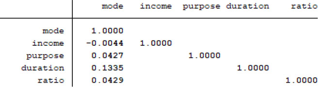
Spearman correlation coefficients for the mode choice model variables.
5.2.2.1. Parameter Estimates
The goal was to employ a model to estimate coefficients within the utility function to ascertain the influence of various individual, household, and excursion characteristics on mode choice. Table 7 presents the z-test results, statistical significance levels, and coefficients for the variables derived from the MNL model estimation, with “private mode” as the base mode. All results are significant at the 95% confidence level.
The model estimation demonstrates statistical signi- ficance, and there is no evidence of multicollinearity within the model, with standard errors of the regression coefficient β not exceeding 0.1. The change in the logit for a one-unit change in the predictor variable is measured by the regression coefficients for the independent variables. In contrast, the other predictor variables remain constant. The transport mode is the dependent variable in this study. It encompasses non-motorized options (walking and bicycle), private transport (van, SUV, car, pickup vehicle), public transport (PT), and taxi (Uber/Lyft). As evidenced by the model results presented in Table 7, the model has been analyzed with a focus on independent variables associated with dependent variables and has statistical significance levels below 0.05.
| Parameter Estimates | |||||||||
|---|---|---|---|---|---|---|---|---|---|
| Transport Mode | Non-Motorized | Public | Taxi | ||||||
| Coeff. | Z-test | P-value | Coeff. | Z-test | P-value | Coeff. | Z-test | P-value | |
| Constant | -0.684 | -48.65 | 0.000 | -1.783 | -79.13 | 0.000 | -3.926 | -76.90 | <0.00 |
| Income 2 | -0.648 | -47.13 | 0.000 | -0.949 | -33.90 | 0.000 | -1.208 | -22.01 | <0.00 |
| Income 3 | -0.707 | -52.26 | 0.000 | -1.112 | -37.60 | 0.000 | -1.043 | -21.13 | <0.00 |
| Income 4 | -0.600 | -41.68 | 0.000 | -1.030 | -31.07 | 0.000 | -0.971 | -16.81 | <0.00 |
| Income 5 | -0.378 | -25.98 | 0.000 | -0.612 | -19.20 | 0.000 | omitted | ||
| Purpose 2 | -0.949 | -77.00 | 0.000 | -0.374 | -13.54 | 0.000 | -0.220 | -3.82 | <0.00 |
| Purpose 3 | 0.629 | 60.66 | 0.000 | omitted | 0.479 | 8.24 | <0.00 | ||
| Purpose 4 | -1.227 | -71.17 | 0.000 | 1.137 | 53.13 | 0.000 | omitted | ||
| Purpose 5 | -0.445 | -46.07 | 0.000 | omitted | 0.102 | 2.18 | <0.00 | ||
| Ratio | -0.574 | -69.58 | 0.000 | -2.737 | -97.80 | 0.000 | -1.400 | -28.56 | <0.00 |
| duration | -0.006 | -32.70 | 0.000 | -0.011 | 78.22 | 0.000 | -0.005 | 11.63 | <0.00 |
| Parameter Estimates | |||||||||
|---|---|---|---|---|---|---|---|---|---|
| Transport Mode | Non-Motorized | Public | Taxi | ||||||
| RRR | Z-test | P-value | RRR | Z-test | P-value | RRR | Z-test | P-value | |
| Constant | 0.505 | -48.65 | 0.000 | 0.168 | -79.13 | 0.000 | 0.020 | -76.90 | <0.00 |
| Income 2 | 0.523 | -47.13 | 0.000 | 0.387 | -33.90 | 0.000 | 0.300 | -22.01 | <0.00 |
| Income 3 | 0.492 | -52.26 | 0.000 | 0.329 | -37.60 | 0.000 | 0.352 | -21.13 | <0.00 |
| Income 4 | 0.549 | -41.68 | 0.000 | 0.357 | -31.07 | 0.000 | 0.379 | -16.81 | <0.00 |
| Income 5 | 0.685 | -25.98 | 0.000 | 0.542 | -19.20 | 0.000 | omitted | ||
| Purpose 2 | 0.387 | -77.00 | 0.000 | 0.688 | -13.54 | 0.000 | 0.803 | -3.82 | <0.00 |
| Purpose 3 | 1.877 | 60.66 | 0.000 | omitted | 1.614 | 8.24 | <0.00 | ||
| Purpose 4 | 0.293 | -71.17 | 0.000 | 3.117 | 53.13 | 0.000 | omitted | ||
| Purpose 5 | 0.641 | -46.07 | 0.000 | omitted | 1.108 | 2.18 | <0.00 | ||
| Ratio | 0.563 | -69.58 | 0.000 | 0.065 | -97.80 | 0.000 | 0.248 | -28.56 | <0.00 |
| duration | 0.994 | -32.70 | 0.000 | 0.989 | 78.22 | 0.000 | 0.995 | 11.63 | <0.00 |
The Relative Risk Ratio (RRR) of a coefficient illustrates the degree to which the risk of the outcome in the comparison group is comparable to the risk of the outcome in the referent group. An RRR greater than 1 indicates that the risk of the comparison outcome in the comparison group relative to the referent group increases as the variable increases, indicating an increased likelihood of the comparison outcome. In contrast, an RRR less than 1 suggests that the risk of the outcome in the comparison group relative to the referent group decreases as the variable increases. Table 8 illustrates the RRR for our alternative-specific MNL model, with “private mode” as the base mode.
The interpretation of the Alternative-Specific Mode Choice model will concentrate solely on the following variables:
- The findings reveal that a one-unit increase in the independent variable “trip purpose 3” (Home-based social/recreational) is correlated with a 0.629 increase in the relative log odds of opting for non-motorized transport and a 0.479 increase in the relative log odds of selecting Taxi transport over private transport. This outcome indicates a preference for non-motorized and Taxi modes for home-based social/recreational trips compared to other transport modes.
- In addition, Table 7 displays the ratio variable of vehicles per household size, which indicates that a one-unit increase in the independent variable is associated with a (0.574, 2.737, and 1.4) decrease in the relative log odds of choosing (non-motorized travel, public travel, and Taxi), respectively, in comparison to private mode. This serves as evidence that the presence of vehicles in a household has a statistically significant impact on the probability of selecting alternative modes of trans- portation compared to private modes.
- The model results suggest that a one-unit increase in the independent variable (income: 2, 3, 4, and 5) is associated with a decrease in the relative log-likelihood of selecting (non-motorized, public, or taxi) modes, as opposed to private transport, for monthly income levels 2, 3, 4, and 5. Consequently, this result implies that an increase in the total household income is correlated with a higher likelihood of travelers selecting private modes of transportation.
- The model results indicate that a one-unit increase in the independent variable of trip duration is associated with a (0.006, 0.011, and 0.005) decrease in the relative log-likelihood of selecting non-motorized, public, and taxi transport, respectively, in comparison to private transportation. This confirms that travelers are more likely to switch from other private transportation modes as the duration of their journey increases.
- The model results also reveal that a one-unit increase in the independent variable “trip purpose-2” (Home-based shopping) is linked to a decrease in the relative log odds of selecting non-motorized, public, or Taxi transport instead of opting for private transport. This suggests that home-based shopping trips are more likely to be undertaken using private transport than other modes.
- The model results also indicate that a one-unit increase in the independent variable “trip purpose-5” (Non-Home-based) correlates with a 0.102 increase in the relative log odds of opting for Taxi transport compared to private transport. This outcome suggests that non-home-based trips are more likely to be undertaken using Taxi transport rather than private modes.
- The model results also demonstrate that a one-unit increase in the independent variable “trip purpose-4” (Home-based work) is correlated with a 1.137 increase in the coefficient for choosing public transport over private transport. This finding suggests that home-based work trips are more likely to be undertaken using public transport rather than private modes.
Based on these findings, we conclude that individual, household, and trip characteristics exhibit a statistically significant influence on the mode chosen in the United States, with notable variations for each variable.
5.2.3. Generic Mode Choice Model
5.2.3.1. Parameter Estimates
We will presuppose that the explanatory variables' coefficients are generic and consistent across alternatives. The parameter estimates of the generic mode choice model are presented in Table 9, with “private mode” as the base mode.
5.2.4. Summary Statistics of the Mode Choice Models
Table 10 provides the summary statistics for both the Generic and Specific mode choice models.
| Parameter Estimates | |||||||||
|---|---|---|---|---|---|---|---|---|---|
| Transport Mode | Non-Motorized | Public | Taxi | ||||||
| Coeff. | Z-test | P-value | Coeff. | Z-test | P-value | Coeff. | Z-test | P-value | |
| Constant | -1.211 | -97.76 | 0.000 | -3.109 | -210.3 | 0.000 | -4.664 | -207.5 | <0.00 |
| Income | -0.011 | -3.91 | 0.000 | -0.011 | -3.91 | 0.000 | -0.011 | -3.91 | <0.00 |
| Purpose | -0.060 | -27.94 | 0.000 | -0.060 | -27.94 | 0.000 | -0.060 | -27.94 | <0.00 |
| Ratio | -0.911 | -112.9 | 0.000 | -0.911 | -112.9 | 0.000 | -0.911 | -112.9 | <0.00 |
| duration | 0.002 | 23.17 | 0.000 | 0.002 | 23.17 | 0.000 | 0.002 | 23.17 | <0.00 |
| Specific Model | Generic Model | |
|---|---|---|
| Number of observations | 819,610 | 819,610 |
| Log likelihood (0) | -368252.95 | -368252.95 |
| Log likelihood (β) | -336243.43 | -359571.37 |
| K (number of parameters including the constant term) | 29 | 5 |
We implement the likelihood ratio test to determine whether a coefficient should be generic or alternative-specific. Here, the Log-likelihood functions of the res- tricted and unrestricted relevance models are compared. The unrestricted model includes alternative-specific coefficients for the four alternatives, whereas the restricted model incorporates generic coefficients. Consequently, the null hypothesis is as follows:
H0 = Generic Coefficients hold
H1= Generic Coefficients do not hold.
and the test statistic for the null hypothesis is given by
 |
With degrees of freedom (df) = KU − KR, where KU and KR are the counts of the estimated parameters in the unrestricted and restricted models, respectively. This is asymptotically distributed as χ 2. We reject the null hypothesis that the restrictions are valid if
−2(LR − LU) > χ2 ((1−α), df)
Where:
α is the level of significance. In this specific case, using α = 0.05 yields:
-2 (- 359571.37 + 336243.43) = 46655.88 > 13.848
Consequently, we can reject the null hypothesis and infer that the coefficients should be alternative-specific. Consequently, the mode choice models are as follows:
V (non-motorized) = – 0.684 – 0.648 (Income 2) – 0.707 (Income 3) – 0.6 (Income 4) – 0.378 (Income 5) – 0.949 (Purpose 2) + 0.629 (Purpose 3) – 1.227 (Purpose 4) – 0.445 (Purpose 5) – 0.574 (Ratio) – 0.006 (duration)
V (Public) = – 1.783 – 0.949 (Income 2) – 1.112 (Income 3) – 1.03 (Income 4) – 0.612 (Income 5) – 0.374 (Purpose 2) + 1.137 (Purpose 4) – 2.737 (Ratio) – 0.011 (duration)
V (Taxi) = – 3.926 – 1.208 (Income 2) – 1.043 (Income 3) – 0.971 (Income 4) – 0.220 (Purpose 2) - 0.479 (Purpose 3) + 0.102 (Purpose 5) – 1.40 (Ratio) – 0.005 (duration)
5.2.4.1. Test of Independency from Irrelevant Alternatives (IIA)
The ‘Hausman & McFadden’ test involves estimating two MNL models: one with the complete choice set (Non-motorized, Private, Public, and Taxi) and the other with a subset of alternatives (Non-motorized, Private, and Public). Fig. (4) illustrates the test results generated using STATA software [23]. Based on these results, we have compelling evidence to accept the null hypothesis, indicating that the Independence from the IIA assumption holds. Therefore, the MNL model is deemed suitable, and there is no need to calibrate an NL regression model.
5.2.5. Mode Choice Model Validation
The previously estimated choice model was developed using approximately 90% trip observations. Consequently, the remaining 10% will be forecasted using the same model. Table 11 presents the estimated, forecasted, and actual probability results of the available modes. The percentage error results provide substantial evidence regarding the quality of the estimated mode choice model. Fig. (5) illustrates the available modes versus the forecasted and actual choice probabilities.
| Available Modes |
Estimated Prob. (~90% of the dataset) |
Forecasted Prob. (~10% of the dataset) |
Actual Prob. (~10% of the dataset) |
Percent Error (Actual-Forecasted/Actual)*100% |
|---|---|---|---|---|
| Non-motorized | 0.099394 | 0.098922 | 0.1045 | 0.56% < 1% |
| Private | 0.882556 | 0.882828 | 0.8773 | 0.55% < 1% |
| Public | 0.014904 | 0.015138 | 0.0156 | 0.05% < 1% |
| Taxi | 0.003146 | 0.003112 | 0.0026 | 0.05% < 1% |
| Sum | 1.000000 | 1.000000 | 1.0000 | ---- |
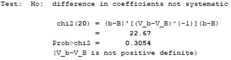
Result of Hausman & Mcfadden test.
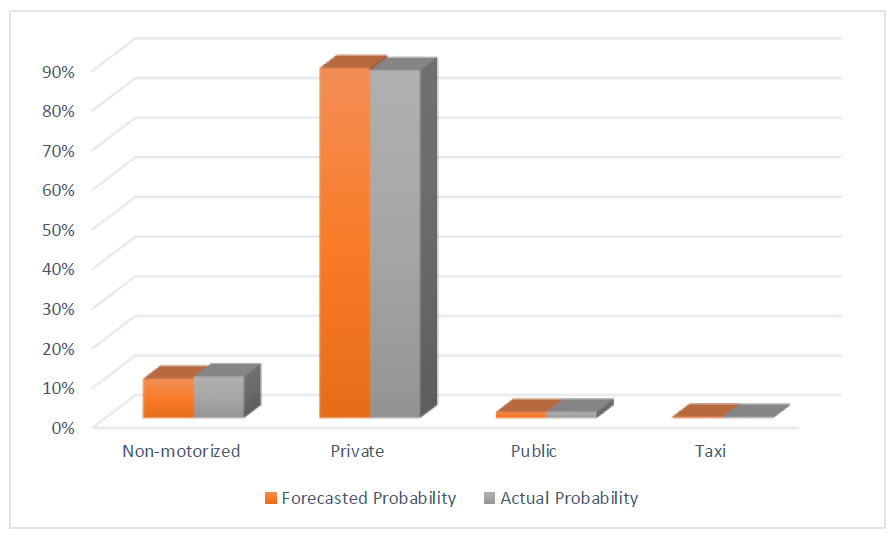
Available modes vs. choice probabilities.
CONCLUSION
Transportation estimation stands as a critical aspect of transportation planning. The significance of accurate traffic forecasting cannot be overstated, as it plays a pivotal role in ensuring the success of the planning process. This study utilized data from the NHTS [21] to calibrate trip generation models and a mode choice model.
Two individual trip-based generation models were employed for weekdays and weekends, allowing for a comparative analysis of factors influencing daily person trips. The differences between the two models were examined, and the relationship between the dependent variable (number of trips) and explanatory variables was estimated using NB regression analysis. The results indicated variations between weekday and weekend models, with the presence of non-workers and individuals' education levels emerging as crucial factors for weekday travel. Conversely, the existence of children, household income level, and personal yearly miles driven were identified as significant factors affecting weekend travel. Additionally, common characteristics such as household size and urban residence were substantial in both models.
Additionally, this investigation aims to evaluate the influence of various variables on selecting a mode of transportation. To accomplish this goal, the MNL regression analysis investigated the correlations between individual, household, activity, and trip characteristics and the modes of transportation selected by travelers. Modeling techniques and testing were implemented to guarantee that the model corresponds to the data per statistical criteria. The variables' estimates were carefully analyzed and interpreted. The primary results indicated that specific variables substantially impact the selection of a mode. The P-value and z-test of variables indicated the statistical significance of all explanatory variables, providing a strong foundation for our findings. Although their effects and contributions varied based on their coefficient values, the statistical significance of all explanatory variables instills confidence in the robustness of our study. Additionally, model validation results provided strong evidence of the high quality of the estimated mode choice model.
In summary, the variables' importance can be determined in the following order: “activity purpose,” “household income,” “ratio of available vehicles to household size,” and “trip duration.” The most significant factors influencing an individual's mode choice are household income, the ratio of available vehicles to household size, and activity purpose.
STUDY LIMITATIONS AND FUTURE DIRECTIONS
This study provides promising insights into individual trip-based generation and mode choice behavior in the United States. However, the study's main limitation lies in modeling techniques. Future research could explore applying more sophisticated models, such as mixed logit or probit models, to enhance the mode choice model. Furthermore, the results may be subject to inherent limitations due to potential shifts in travel behavior. In the future, it would be advantageous to rerun the models on updated and comprehensive datasets, allowing for continuous validation and adaptability over time.
Additionally, while this research utilizes data from the NHTS, the methodology applied in this study is flexible. It can be replicated using updated versions of this dataset or similar travel surveys from future years. This adaptability ensures the model's relevance in evolving contexts and its potential application to a broader range of scenarios, further enhancing methodological replicability.
Another limitation relates to the dataset size, as the filtering procedure necessitated excluding numerous trips due to incomplete data. Future research should focus on an extended analysis to comprehensively identify a broader range of variables influencing mode choice. Expanding the scope of these variables will provide a deeper understanding of the factors shaping travel decisions.
Moreover, conducting a zonal analysis with a larger dataset could facilitate the development of more accurate zone-based trip generation models, offering insights into localized travel behavior patterns. Integrating real-time data sources, such as GPS or mobile app data, into the models will help refine them by capturing emerging trends and offering a more dynamic perspective. Incorporating environmental factors, such as weather conditions and emissions, will further enrich the analysis, enabling a more holistic understanding of how to promote sustainable and eco-friendly mobility solutions.
AUTHORS’ CONTRIBUTION
B.Q., Conceptualization; S.Q.: methodology; B.Q. & A.T.: formal analysis; D.Q.: investigation; B.Q. & D.Q.: resources; S.Q.: data curation; B.Q., D.Q., S.Q., A.T.: writing—original draft preparation; B.Q.: writing—review and editing.
LIST OF ABBREVIATIONS
| NB | = Negative Binomial |
| MNL | = Multinomial Logit |
| NHTS | = National Household Travel Survey |
| FHWA | = Federal Highway Administration |
| NL | = Nested Logit |
| IIA | = Irrelevant Alternatives |
| CV | = Continuous Variable |
| DV | = Dummy Variable |
| IV | = Indicator Variable |
| IRR | = Incidence Rate Ratio |
| RRR | = Relative Risk Ratio |

