All published articles of this journal are available on ScienceDirect.
Assessing Non-linear Influences of Urban Layout on Driving Travel Distance: A Mumbai Case Study
Abstract
Introduction
This study investigates the impact of built environment factors on travel behavior in Mumbai, India, focusing on the non-linear effects on driving distances. The rapid urbanization and complex urban of Mumbai constitute present challenges for sustainable transportation, necessitating a deeper understanding of how urban planning influences travel behavior. While demographic factors have often been highlighted in travel studies, this research prioritizes the role of built environment factors.
Materials and Methods
The study utilized Gradient Boosting Decision Trees (GBDT) to analyze household travel survey data from Mumbai, capturing the non-linear relationships between built environment variables and driving distances. Partial dependence plots were used to visualize these effects, and the relative importance of each variable was assessed to identify key determinants of travel behavior.
Results
The analysis identified trip time as the most influential factor in determining driving distances, followed by built environment characteristics, such as proximity to commercial areas and intersection density. Socio-demographic factors were found to have a comparatively low impact. Non-linear relationships were observed, such as the stabilization of driving distances beyond certain thresholds of block density and proximity to bus stops.
Discussion
The findings challenge the traditional emphasis on demographic factors in explaining travel behavior, highlighting the significant role of urban form. The study reveals that specific built environment factors, such as accessibility and connectivity, play a crucial role in shaping driving behavior in a rapidly urbanizing city like Mumbai. These results suggest that urban planning strategies should prioritize these factors to reduce car dependency.
Conclusion
This study underscores the importance of the built environment in influencing travel behavior in Mumbai, particularly in reducing driving distances. The insights gained offer valuable guidance for urban planners and policymakers aiming to promote sustainable mobility in rapidly developing cities. Further research is recommended to validate and expand upon these findings in other urban contexts.
1. INTRODUCTION
Rapid urbanization in developing countries has led to significant changes in the built environment, influencing travel behavior and distances traveled using various modes of transportation. While this relationship has been extensively studied in contexts like North America, Europe, and China [1-7], there is a lack of research focusing on rapidly urbanizing cities in developing countries like India. This study aims to bridge this gap by utilizing household travel survey data from the Mumbai Metropolitan Region (MMR) to offer new insights into the interactions between urban form and travel distances for active travel modes.
Specifically, the key objectives of this research are: (i) to quantify the relative influence of built environment factors versus demographic factors on driving distances in Mumbai; (ii) to identify critical thresholds and effective ranges for built environment parameters significantly impacting driving distance. By employing the advanced machine learning technique of gradient boosting decision tree (GBDT) and leveraging non-linear modeling capabilities, this study aims to capture the relationships between the built environment and travel behavior in the rapidly urbanizing context of Mumbai. The insights gained will contribute to a deeper understanding of these dynamics in developing countries, informing data-driven urban planning and transportation policies to promote sustainable mobility solutions tailored to unique local contexts.
Earlier studies have examined the combined influence of the built environment and commuting initiatives on the selection of transportation modes for work [8] in Washington, as well as the effects of property accessibility and the surrounding built environment on the valuation of residential properties [9] in China. Additionally, research in South India has been conducted on the connection between the design of urban spaces, environmental pollution, and public health [10] and on how neighborhood choices and the built environment sway patterns of physical commuting [11]. Further inquiries have explored residential self-selection and decision-making processes within the framework of the built environment, alongside considerations of travel disposition and patterns [12]. The variances in choices of transportation modes and the sequencing of trips during holiday periods as opposed to regular weekdays have also been a subject of analysis [13]. While previous studies have often relied on traditional regression methods to explore the relationship between the built environment and travel behavior, these techniques may fail to capture the complex, non-linear dynamics that characterize rapidly urbanizing regions like Mumbai. This study introduces a novel approach by utilizing Gradient Boosting Decision Trees (GBDT), a machine learning technique that excels in modeling non-linear relationships and interactions among variables. By applying GBDT, we aim to provide a more nuanced understanding of the built environment's influence on travel behavior in developing countries, contributing to more effective urban planning strategies.
Building upon these findings, our study aims to quantify the influence of built environment factors on the active distance traveled relative to demographic factors in Mumbai. Moreover, this research analyzes the varying effects of urban infrastructure on active travel distance compared to recreational journeys, highlighting the need for customized urban development approaches. The findings of this study, which is the first to use household travel survey data from the Mumbai Metropolitan Region (MMR), can guide data-driven urban planning and transportation policies in fast-developing regions of developing countries.
In this study, we examine a comprehensive set of demographic and built environment factors that potentially influence driving distances in Mumbai. Demographic factors include age, income, gender, and driving license status. Built environment factors encompass the “5Ds” framework: density (e.g., block density, intersection density), diversity (e.g., entropy index for land use mix), design (e.g., street connectivity), destination accessibility (e.g., distance to commercial areas, CBD), and distance to transit (e.g., proximity to bus stops and railway stations). We also consider trip characteristics, such as trip time and cost. By employing GBDT, we aim to identify critical thresholds and effective ranges for these parameters. For instance, we explore how driving distances change with varying levels of intersection density, land use diversity, or proximity to transit nodes. These thresholds and ranges, such as the optimal distance to commercial areas or the impact of different levels of land use mix, provide actionable insights for urban planners and policymakers. Our analysis reveals non-linear relationships between these factors and driving distances, highlighting the complex dynamics at play in Mumbai's urban environment.
The organization of this document is as follows: Section 2 reviews prior studies examining the nexus of the built environment and transportation patterns, focusing on three pivotal inquiries. Section 3 delineates the approach for modeling. Section 4 presents an exhaustive exami- nation of the dataset and the variables in question. The subsequent segment addresses the inquiries posited by the research. Concluding the paper, the principal discoveries are encapsulated, and their relevance to urban development is discussed.
2. LITERATURE REVIEW
2.1. The Built Environment and Travel Behavior: An Overview
The built environment, encompassing urban form elements such as density, diversity, design, destination accessibility, and distance to transit (the “5Ds”), has been widely studied for its influence on travel behavior (Ewing & Cervero, 2010). Urban form refers to the physical characteristics of urban areas, while the built environment is a broader term that includes both natural and constructed elements shaping human activity patterns [14]. Research has consistently shown that denser, more diverse, and well-connected urban environments are associated with reduced automobile dependence and increased use of sustainable transport modes [15-17]. However, the magnitude and nature of this relationship remain subjects of debate.
A study [18] found that while individual built environment factors have modest effects on travel behavior, their cumulative impact is significant. In contrast, another [19] argued that urban form has only marginal influences on commuting patterns, cautioning against overvaluing environmental changes. This sparked further debate, with other studies [3, 20] critiquing Stevens' methodology and emphasizing the benefits of compact development. The relative influence of urban characteristics versus personal traits on travel patterns is a key focus of another research [21]. Some studies suggest that urban layout impacts vehicle miles traveled (VMT) or vehicle hours traveled (VHT) more significantly than demographic factors [22, 23]. However, others argue that demographic characteristics and residential self-selection play a more crucial role [24, 25].
2.2. Machine Learning Insights into Built Environment and Travel Dynamics
Machine learning techniques have increasingly been applied to examine the complex, often non-linear relationships between the built environment and travel behavior. These methods offer several advantages over traditional regression approaches, including the ability to capture non-linear relationships, handle high-dimensional data, and reveal variable importance. Recent applications of machine learning in this field include a study [26] that used random forests to predict travel behavior, finding that urban factors account for about half of the behavioral variance. Another study [8] employed Gradient Boosting Decision Trees (GBDT) to assess urban structures' impact on driving patterns, explaining up to 65% of the variance. Another study [7] utilized GBDT to show that urban form factors significantly predict active travel, accounting for nearly 69% of predictive accuracy. These studies demonstrate the potential of machine learning to provide deeper insights into the complex interplay between the built environment and travel behavior. However, it is important to note that while machine learning offers powerful analytical capabilities, it should be used in conjunction with domain knowledge and careful interpretation to ensure meaningful results.
2.3. Recent Findings and Research Gap on Built Environment and Travel Bahaviour
Recent studies have provided nuanced insights into the relationship between the built environment and travel behavior across various contexts. In developed countries, findings show that the built environment modestly affects commuting distance but significantly impacts mode choice, such as in France and Australia [27, 28]. In developing countries, research reveals complex, non-linear relationships between urban form and travel behavior, with high-density areas reducing car dependency but road density exhibiting non-linear effects on car use, as seen in China [29]. Similarly, in Ghana, a polycentric urban structure influences commuting patterns, with socio-economic factors playing a significant role [30]. Despite extensive research, significant gaps remain. Socio- economic factors, such as age, gender, education, and income, delineate distinct travel behavior patterns. Higher-income groups experience more pronounced effects of urban infrastructure on walking behavior.
Additionally, urban infrastructure’s impact varies between work-related and non-work-related trips, with land use variety promoting non-work-related active travel [31-33]. These gaps are particularly evident in rapidly urbanizing regions like India, where traditional regression methods may not capture complex relationships. Therefore, the use of advanced machine learning tech- niques, such as Gradient Boosting Decision Trees (GBDT), offers deeper insights, challenging the legitimacy of linear models.
2.4. Key Research Questions and Objectives
1. What is the relative influence of built environment factors versus demographic variables on travel behavior in rapidly urbanizing regions?
2. What are the critical thresholds and effective ranges for built environment parameters that significantly impact travel patterns?
By addressing these questions, the study aims to quantify the relative influence of the built environment versus demographic factors on travel distances and to identify specific urban parameters with significant impacts on driving behavior in Mumbai. This knowledge can inform urban planning and transportation policies tailored to developing countries, promoting sustainable mobility solutions.
3. METHOD
The study introduces gradient-boosting decision trees (GBDT), a model that predicts outcomes by optimizing a loss function and integrating principles from statistics and machine learning [34]. Unlike traditional regression models, GBDT handles various independent variable types with minimal preprocessing, manages missing values, and is resilient against outliers. It naturally captures non-linear dynamics and interactions between variables [35]. GBDT excels in identifying variations in traveled distance, enhancing predictive precision through boosting. It outperforms conventional methods, including regression, ARIMA, RF, NN, and SVM models [36-38]. Despite its strengths, GBDT does not consider the causal sequence among independent variables. For instance, it does not assess the statistical significance of the influence of a neighborhood's proximity to the city center on population density. However, GBDT provides valuable insights into these relationships, outperforming conventional linear analyses. The next section will detail the GBDT algorithm mathematically.
3.1. Gradient Boosting Decision Trees
This study employs Gradient Boosting Decision Trees (GBDT) due to their capability to capture complex, non-linear relationships between the built environment and travel behavior. Unlike traditional regression models, GBDT can handle high-dimensional data and interactions among variables, offering a more accurate and detailed analysis. This methodological approach represents a significant advancement in urban studies, particularly in rapidly urbanizing cities like Mumbai, where traditional models may oversimplify the relationships between urban form and travel patterns. This machine learning technique [34, 39] has been increasingly adopted in studies related to the built environment and travel behavior [40, 41]. It combines decision trees with gradient boosting. A decision tree employs a hierarchical structure to segment a sample into multiple subsamples based on specific criteria, using the mean of the dependent variable within each subsample for prediction. However, a single decision tree often yields poor predictions. In contrast, gradient boosting enhances the model by iteratively combining the outcomes of simple decision trees into a more robust model.
The notation, first brought to light in a previous study [34] and subsequently adapted into an R package by (Ridgeway, 2024), utilizes Xi, Yi to signify the ith sample in the sample space S, which encompasses N samples. In this scenario, Xi is the array of independent variables, and \Yi is the dependent variable. Additionally, X is the matrix of independent variables spanning all samples.
Before model estimation, the GBDT framework requires the definition of three parameters: tree depth (K), learning rate (λ), and the number of iterations (T). The process commences by initializing a constant  = argmin
  where Ψ denotes the loss function and ρ signifies the ideal parameter. The procedure will be repeated for T iterations. During the ith iteration, the initial step involves employing Eq. (1) to ascertain the negative gradient zi for the ith data point.
 |
(1) |
Step 2 entails constructing a decision tree with K terminal nodes using a subset of the data. Earlier research [39] highlighted the advantages of constructing decision trees using a subset randomly chosen from the full dataset, which demonstrated improved results. The recommendation was that this subset should include half the number of observations in the dataset, represented as 0.5 × N observations (Eq. 2).
 |
(2) |
SK represents the set of observations classified into the kth terminal node of the decision tree fitted in Step 2. Step 4 involves updating  utilizing Eq. (3):
 |
(3) |
Eq. (3) designates K(X) as the marker of the end node in the decision tree where the data points reside. In numerous facets, Gradient Boosted Decision Trees (GBDT) outperform traditional statistical models like linear regression and generalized linear models.
Firstly, GBDT excels in capturing intricate and non-linear associations among variables efficiently without relying on predefined relationships. Unlike traditional models constrained by linearity assumptions, which often necessitate transformations to accommodate nonlinearity, the flexibility of GBDT enables it to adapt to any form of nonlinearity seamlessly [42].
Secondly, GBDT demonstrates adeptness in handling missing data and outliers in predictors. Unlike conven- tional methods that may remove observations with missing values and risking biased parameter estimates, decision trees address this issue by aggregating instances with missing data into one subset during splitting [43]. Moreover, decision trees base their splits solely on variable rankings, diminishing the impact of outliers and preserving a larger sample for model training [43]. Third, Gradient Boosting Decision Trees (GBDT), as a method grounded in tree-based algorithms, excel in forecasting outcomes with greater precision by effectively discerning complex non-linear patterns (Grinsztajn et al., 2022). Studies examining the link between constructed surroundings and travel patterns uniformly recommend tree-based approaches as superior to alternative methodologies [7, 44, 45]. Despite the numerous advantages of the GBDT method, it is not devoid of limitations. Initially, it lacks the provision of p-values necessary for statistical inference. Instead, this study depends on evaluating the practical significance of independent variables through scales of relative importance and influence. Secondly, GBDT is susceptible to overfitting, a challenge we tackled by implementing cross-validation during model estimation.
The computational estimations were performed utilizing the “gbm” package in R, as per [46]. The model's construction involved the specification of three crucial parameters: the depth of the tree, the learning rate, and the total number of trees. The tree's depth, denoted by a positive whole number, reflects the intricacy of the decision tree's configuration. Although deeper trees augment data fitting, they simultaneously elevate the potential for overfitting. The learning rate, which varies between 0 and 1, dictates the fraction of decision tree estimates that are integrated into the final model. A reduced learning rate enhances performance but demands additional computational resources. The quantity of trees specifies the count of decision trees incorporated in the final model. While a higher number of trees boost data fitting, they also intensify the overfitting risk in alignment with the research methodologies established by a previous study [41, 47].
GBDT techniques offer an interpretable structure by quantifying the significance of each predictor and delineating the associations between dependent and independent variables. Within the scope of the “gbm” package, the relative importance metric quantifies the influence of an independent variable on the prediction of the dependent variable. This metric signifies the fraction of variance reduction attributed to a specific independent variable in comparison to the total variance reduction achieved by all predictors. Being a normalized measure, relative importance aids in comparing the effects of different built environment factors on diverse travel behaviors. The following flowchart, as shown in (Fig. 1) illustrates the key steps involved in the Gradient Boosting Decision Trees (GBDT) model employed in this study:
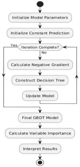
Flowchart of the gradient boosting decision trees (GBDT) process.
3.2. Relative Importance of Influential Factors
Gradient-boosting decision trees (GBDT) theoretically handle various independent variables, identifying their interactions and delineating complex nonlinear relation- ships [35]. It is beneficial to determine the relative significance or influence of each independent variable on the predicted outcome. However, the goals of precision and clarity in predictive modeling are not always aligned [48]. Unlike other machine learning algorithms, such as RF, NN, and SVM, GBDT has the distinct capability to discern and prioritize the effects of independent variables on the forecasted response.
In this study, the predictor xk refers to one of the independent variables within the GBDT model, which is used to split the data into different nodes in the decision trees. The contribution of each predictor, including xk, is incorporated into the model through the updates in Eq. (3), where the term ρk(X) represents the influence of the predictor on the terminal node of the tree. The relative importance of () is then quantified using Eq. (4), where the reduction in squared error due to xk at each internal node is summed across all trees in the ensemble. This provides a measure of how influential xk is in predicting the outcome, as further detailed in Eq. (5).
For a given decision tree (T), earlier research [49] proposed the subsequent metric as a gauge for the relative importance of the predictor xK in the prediction of the response, as shown in Eq. (4):
 |
(4) |
The summation includes the internal nodes t of the J-terminal node tree T, where xk denotes the splitting variable linked to node t, and  represents the empirical reduction in squared error when predictor xκ is utilized as the splitting variable at the internal node t. For an ensemble of decision trees
  obtained via the gradient boosting method, Eq. (4) can be extended by taking the average across all the additive trees, as shown in Eq. (5):
 |
(5) |
4. DATA AND VARIABLES
Mumbai Metropolitan Region (MMR) in India was selected for this investigation as a study area (Fig. 2) known for its vibrant economy and complex socio-economic fabric. It contains Thane, Mumbai City, Raigad, and Mumbai Suburban. As per the data from the 2011 Census, the Mumbai Metropolitan Region (MMR) had a populace of 21.3 million, and it is anticipated to escalate to approximately 34 million by the year 2031. The MMR is home to one-third of the inhabitants of the entire area. Given its population density of about 20,500 people per square kilometer, MMR encounters a range of urban difficulties while also presenting prospects for develop- ment and advancement.
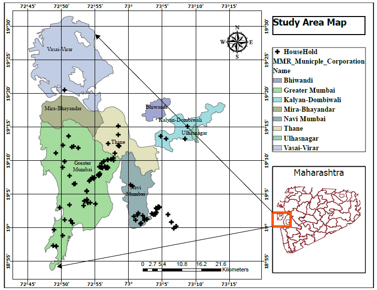
Illustrates the geographical arrangement of the (MMR) and the distribution of the sample [51].
This investigation incorporates a trio of data categories: travel behavior data, which delineates the mode of transport selected by participants; socio- demographic data, detailing their socioeconomic and demographic profiles; and built environment (BE) data, reflecting Mumbai's land use diversity and transit systems. The commuting behavior with sociodemographic infor- mation was derived from a previous study [50].
The data utilized in this study originate from a household travel survey conducted by previous researchers [51]. This survey collected information on demographics, household characteristics, and travel behaviors from 126 households for 15 days, focusing primarily on weekdays to capture routine trip frequencies and activities. The survey was administered using a stratified random sampling method to ensure representative sampling across different socioeconomic strata of Mumbai. Households were selected based on geographic location to cover diverse areas with varying built environment characteristics. The mode of delivery was a self-administered paper survey, distributed and collected by trained field staff who assisted res- pondents when necessary. The survey included detailed instructions and was designed to be user-friendly to minimize response errors. Follow-up visits were conducted to ensure high response rates and data accuracy. The dataset included data from 347 individuals within these households, documenting 21054 trips, with 5891 trips done using different (private cars (as a driver or passenger) and taxi) modes. These trips were categorized into home-based and non-home-based, with particular emphasis on the latter to assess the impact of urban design elements.
It is important to address the representativeness of our sample in relation to Mumbai's large population. While our sample of 126 households (347 individuals) may seem small compared to Mumbai's 21.3 million residents, several factors support its significance and validity. Firstly, the depth of data collected – 21,054 trips over a 15-day period – provides rich, longitudinal information that captures day-to-day variations in travel behavior. The use of stratified random sampling ensures representation across different socioeconomic strata and geographic areas. Moreover, our sample size aligns with other studies in the field of travel behavior, particularly those focusing on specific travel modes or demographic groups [51-54]. The focused nature of our study, examining 5,891 trips made by private car and taxi, allows for detailed analysis of particular travel behaviors. While a larger sample would potentially increase precision, our current sample size is sufficient to detect meaningful effects, especially given our use of advanced methods like Gradient Boosting Decision Trees. Lastly, the resource-intensive nature of collecting high-quality travel data necessitates a balance between depth of information and feasibility, which our 15-day survey period achieves.
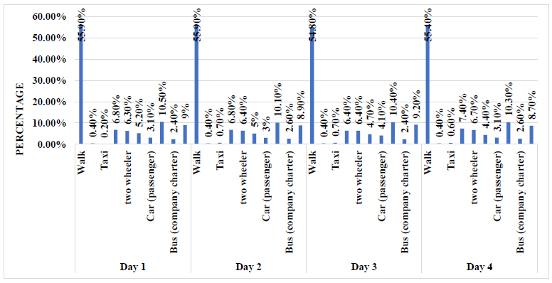
Depicts the relative usage frequencies of different transportation methods throughout the survey [52].
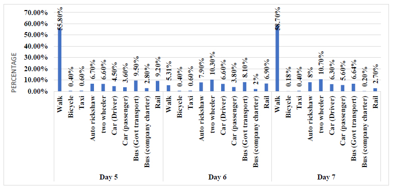
Depicts the comparative frequencies of different transport modes used throughout the research period [52].
In this research, the dependent variable is a binary dummy variable (0, 1), where '1' signifies the completion of a trip using different (a private car (as a driver or passenger) and taxi) modes, while '0' encompasses all other modes. The independent variables are categorized into three clusters: trip characteristics (e.g., distance, duration, and cost), socio-demographic characteristics (e.g., gender, vehicle ownership, age, occupation, and education), and built environment attributes (e.g., number of bus stops, land use mix, intersection density, and proximity to the city center and railway stations). Figs. (3 and 4) present a breakdown of the mode share for each day of the week, providing insights into the travel patterns. Furthermore, Fig. (5) illustrates the proportion of daily trips specifically for work purposes compared to other types of trips.
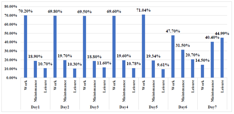
The distribution of trip types (work, maintenance, and leisure) across different days of the week (day 1 through day 7) [52].
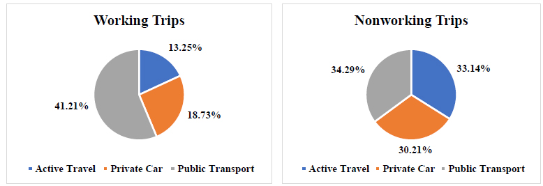
Mode share of working and nonworking trips [52].
Fig. (6) presents the mode share for working and nonworking trips. We can observe distinct patterns in transportation preferences. For working trips, there is a significant reliance on public transport, which accounts for 41.21% of the mode share, while private cars (18.73%) and active travel (13.25%) are less utilized. In contrast, the mode share for nonworking trips is more evenly distributed among the three modes of transportation, with active travel (33.14%) and private car usage (30.21%) notably higher than in the working trips scenario, while public transport (34.29%) remains important but less dominant.
Table 1 provides an overview of the socio-economic characteristics of the surveyed individuals in the Mumbai Metropolitan Region. The survey findings reveal that out of 346 respondents, 31.49% owned one car, 2.36% owned two cars, and the majority (65.35%) did not own any vehicle. In terms of gender distribution, 46.1% of the respondents were female, while 53.9% were male. The predominant level of education achieved was a graduate degree, representing 28.2% of participants. In terms of occupation, students constituted the largest segment at 25.93%, followed by managers at 8.3%. The distribution of income showed a tendency towards the upper echelons, with 17.64% of individuals receiving a monthly income ranging from 10,000 to 20,000 and 17.46% having a monthly income exceeding 100,000.
In this study, we systematically gathered a comprehensive range of potential factors for each data point, as delineated in Table 2. This compilation encom- passes socio-economic variables that encompass both personal and household characteristics. Our study aims to integrate socio-economic and built environment variables to evaluate their influence on the prevalence of active travel. Through an extensive methodological approach, we delve into the diverse elements that may inform a person's choice of transport, thereby clarifying the relationship between the examined variables and the propensity to opt for active travel methods, such as walking or cycling.
| Variable | Description |
|---|---|
| Car Ownership | One car (31.49%) |
| Two cars (2.36%) | |
| No vehicle (65.35%) | |
| Gender | Male (53.89%) |
| Female (46.1%) | |
| Age | <= 18 (20.10%) |
| 19 – 30 (20.46%) | |
| 31 – 40 (25.07%) | |
| 41 – 50 (20.1%) | |
| 51 – 60 (9.79%) | |
| >= 61 (4.3%) | |
| Education Level | Low (Illiterate, Primary 5th pass, Higher Secondary 12th pass) 59.1% |
| Middle (Graduation 28.2%) | |
| High (post-graduation and above 17.5%) | |
| Monthly Income | < 30000 (33.45%) |
| 30001- 100000 (35.65%) | |
| >100000 (17.46%) | |
| No. Driving License | No (28.5%) |
| Yes (71.35%) | |
| Bicycle ownership | Yes (21.42%) |
| No (78.57%) |
| Variable | Mean | Std. Deviation |
|---|---|---|
| Gender | 1.461 | 0.499 |
| Driving license status | 0.853 | 1.253 |
| Car Own | 0.360 | 0.532 |
| TW Own | 0.542 | 0.650 |
| Bicycle Own | 0.017 | 0.131 |
| Education Level | 1.755 | 0.734 |
| Income | 1.816 | 0.714 |
| Job | 4.061 | 2.145 |
| Age Category | 2.919 | 1.412 |
| Driving Trip Time (min) | 11.590 | 33.53 |
| Driving Trip Cost (INR) | 5.84 | 20.41 |
| Public Trip Time (min) | 13.97 | 26.069 |
| Public Trip Cost (INR) | 1.8242 | 7.87 |
| Active Trip Time (min) | 26.089 | 38.583 |
| Active Trip Cost (INR) | 7.666 | 21.389 |
| Built Environment Variables | ||
| Block Density (building/km2) | 307.487 | 200.618 |
| Bus Stop Count | 36.401 | 25.360 |
| Entropy Index | 0.595 | 0.591 |
| Intersection Density | 263.325 | 83.387 |
| Distance to nearest Commercial Area (m) | 471.578 | 235.859 |
| Distance to CBD (m) | 18579.950 | 8133.60 |
| Distance to the railway station (m) | 3463.289 | 3585.943 |
| Distance to nearest Bus Stop (m) | 641.692 | 2300.443 |
| Dependent Variables | ||
| Driving Trip Distance (m) | 5.62 | 17.25 |
| Public Trip Distance (m) | 6.834 | 13.55 |
| Active Trip Distance (m) | 12.609 | 20.079 |
4.1. Built Structure Variables
The urban landscape, or built environment, encompasses human-made structures like land use, transportation networks, and urban design features that influence a multitude of activities and travel decisions. This complexity is often distilled into the “5Ds” framework —density, diversity, design, destination accessibility, and distance to transit, which are pivotal in shaping travel behavior [18, 55]. This research delves into six principal indicators: density, design, diversity, destination accessibility, transit access, and demand management strategies, while excluding certain travel demand measures like parking management and congestion pricing. The neighborhood-level built environment is evaluated using QGIS software and OpenStreetMap data, focusing on eight variables that significantly impact travel mode choice [56].
Diversity in urban layouts is assessed through land use diversity and balance indices. Instead of the traditional job-to-household ratio, modern methods use the entropy index to measure land use heterogeneity and the dissimilarity index for evenness, as well as evaluate the balance between retail and residential spaces or the ratio of job opportunities to retail facilities [57]. Urban design has evolved to emphasize various metrics, such as the inclusion of bicycle lanes for eco-friendly transport systems, and other measures like street-to-block ratios, intersection density, sidewalk width, and parking layouts, which are key to understanding urban density, connectivity, accessibility, expansion, and pedestrian dynamics [58, 59].
| Variable | Description | Mean | Std. Deviation |
|---|---|---|---|
| Block Density (buildings/km2) | The variable represents the amount of buildings per area (building/km2) inside the 1000 m buffer zone. | 307.49 | 200.618 |
| Bus Stop Counts | The variable denotes the count of bus stops inside the 1000 m buffer zone. | 36.40 | 25.360 |
| Entropy Index | The variable signifies the range of urban activities. We categorized urban activities into nine primary types: recreational and amusement, lodging, healthcare, governmental administration, transportation, educational pursuits, commercial ventures, financial operations, and dining establishments. | 0.60 | 0.591 |
| Intersection Density / km2 | The density of street intersections within a community (unit: 1 km2). | 263.33 | 83.387 |
| Distance to nearest Commercial Area (m) | The variable donates to the shortest distance to the nearest commercial area from the respondence home. | 471.58 | 235.859 |
| Distance to CBD (m) | The variable donates to the shortest distance to the CBD from the respondence home. | 18579.95 | 8133.608 |
| Distance to the railway station (m) | The variable donates to the shortest distance to nearest the railway station from the respondence home. | 3463.29 | 3585.943 |
| Distance to nearest Bus Stop (m) | variable donates to the shortest distance to the nearest to the bus stop from the respondence home. | 641.69 | 2300.443 |
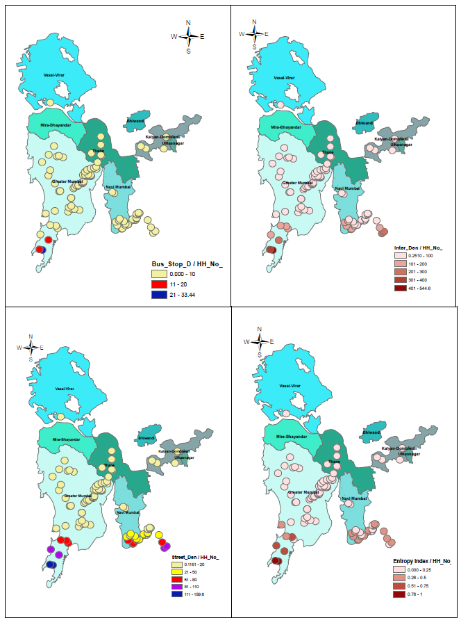
Geographical distribution of the bus stop density, Intersection density, street density, and Land use mix around households within a 1000 m buffer zone [52].
Metrics assessing urban accessibility include proximity to the Central Business District (CBD), indicative of urban centrality and vibrancy, and the evaluation of access to employment centers by car and public transit effective- ness, which are essential for understanding urban travel patterns and promoting sustainable commuting [60]. The evaluation of urban transit accessibility includes metrics like the network distance to transit stops and the walking time to them, which are important for discussions on pedestrian access and urban walkability. The spatial density of transit stops and routes provides insights into service extent and coverage [57]. Demand management in transport policy seeks to regulate private car use by increasing costs and enhancing public transport attractiveness with park-and-ride facilities and infra- structure for pedestrians and cyclists. Assessing how transit-centric neighborhood designs affect transportation choices is crucial [61]. The built environment variables under study are outlined in Table 3. Fig. (7) represents the special distribution of built environment indicators in the study area.
5. RESULTS AND DISCUSSION
Ensuring transparency and reproducibility in machine learning models is crucial for advancing scientific research. To this end, we report the specific hyper- parameter values used for training the Gradient Boosting Decision Trees (GBDT) models on the driving, public transport, and active travel datasets (Table 4). The variations in hyperparameters, such as the maximum tree depth, learning rate, and number of boosting rounds, reflect the careful tuning process undertaken to optimize performance for each travel mode's unique character- istics. The tree depth (K) was set to 6 based on the complexity of the relationships between the built environment factors and travel behavior. This depth was selected after conducting cross-validation experiments, where increasing tree depth beyond 6 showed diminishing returns in model accuracy and increased risk of overfitting. A tree depth of 6 allows the model to capture non-linear relationships effectively without becoming overly complex. The learning rate (λ), set to 0.1, provided a good balance between model convergence speed and accuracy. A lower learning rate would have required more iterations to reach optimal performance, increasing computational costs, while a higher rate could lead to suboptimal convergence. Cross-validation was used to ensure this learning rate efficiently minimized the loss function.
The number of iterations (T), set to 100, was determined through early stopping criteria during the cross-validation process. By monitoring the model’s performance on a validation set, we ensured that the model was trained with sufficient boosting rounds to achieve high accuracy while avoiding overfitting. This number of iterations allowed the model to converge to an optimal solution without excessive computational costs. For instance, the deeper trees (max depth = 6) employed for the model suggest that more complex decision boundaries were required to capture the non-linear relationships effectively. Consistent techniques like column and row subsampling were applied across all models to improve generalization. Providing these hyper- parameter values not only enables reproducibility but also offers insights into the models' behavior, facilitating interpretation and benchmarking for future studies in travel behavior modeling using machine learning techniques.
| Hyperparameters | Driving |
|---|---|
| N rounds | 100 |
| Max depth | 6 |
| Eta | 0.1 |
| Gamma | 0 |
| Col sample by tree | 1 |
| Min child weight | 1 |
| subsample | 0.5 |
5.1. Relative Importance of Independent Variable
One common approach for interpreting machine learning models involves assessing relative importance. In Gradient Boosting Decision Trees (GBDT), this is achieved by iteratively selecting independent variables to build individual decision trees, with the frequency of selection indicating relative importance [34, 62]. The resulting relative importance is shown in Table 5, where values are scaled so that the sum across all variables equals 100%. Higher relative importance values suggest greater contributions to successful predictions [37].
The findings from this study offer valuable insights into the intricate relationships between the built environment and travel behavior in the rapidly urbanizing context of Mumbai, India. By employing the advanced machine learning technique of Gradient Boosting Decision Trees (GBDT), we were able to capture the non-linear dynamics governing the distances traveled by driving. Our results align with previous research highlighting the significant influence of urban form on travel patterns [15-17, 63, 64]. Echoing the findings of [18], we observed that various elements of the built environment, collectively termed the “5Ds” (density, diversity, design, destination accessibility, and distance to transit), exerted a substantial impact on travel behavior. The results revealed striking patterns in terms of the relative importance of different factors influencing travel distances. For driving, trip time emerged as the overwhelming determinant, with a relative importance value of 90.49%. This finding underscores the universal desire to minimize commuting time, a phenomenon consistent with the principle of stable travel time budgets [65]. The overwhelming importance of trip time aligns with previous studies that have identified it as a critical determinant of travel choices [23, 66].
For driving distances, after trip time, the distance to the nearest commercial area (1.15%) and the distance to the central business district (CBD) (1.02%) emerged as
| Variables | Driving Model | |
|---|---|---|
| Relative importance % | Rank | |
| Trip characteristic | ||
| Trip Cost | 2.11 | 2 |
| Trip Time | 90.49 | 1 |
| Socio-demographics | ||
| Age | 0.80 | 6 |
| Income | 0.080 | 15 |
| Gender | 0.175 | 14 |
| Driving license status | 0.2731 | 12 |
| Job | 0.248 | 13 |
| TW Own | 0.0099 | 17 |
| Car Own | 0.008 | 18 |
| Bicycle Own | 0 | 19 |
| Education | 0.063 | 16 |
| Built environment | ||
| Distance to nearest Bus Stop | 0.458 | 11 |
| Entropy Index | 0.58 | 8 |
| Bus Stop Count | 0.48 | 9 |
| Distance to nearest Commercial Area | 1.151 | 3 |
| Block Density | 0.473 | 10 |
| Intersection Density | 0.923 | 5 |
| Distance to CBD | 1.0181 | 4 |
| Distance to Railway station | 0.638 | 7 |
significant built environment factors, echoing the findings of a previous study [67-69], which highlighted the importance of proximity to employment centers and amenities. Additionally, intersection density (0.92%), a measure of street connectivity and urban design, played a crucial role, corroborating previous findings [6]. Interestingly, our analysis revealed that socio-demographic factors played a relatively minor role in influencing travel behavior for driving, with age, income, gender, and driving license status showing low relative importance values. This divergence from some previous studies that emphasized the significance of demographic factors [25, 66] may be attributed to the unique urban context of Mumbai, as well as the robust analytical approach employed, which effectively isolated the influence of built environment characteristics.
These findings contribute to the ongoing debate regarding the relative influence of urban form and demographic factors on travel patterns. While some scholars argue that demographic factors outweigh urban form in explanatory capacity [25], our results align more closely with the perspectives of a previous study [23], suggesting that urban planning elements exert a more substantial effect on travel behavior than individual demographic characteristics. It is important to note that the interpretations presented here are specific to the context of Mumbai, a rapidly urbanizing city in a developing country. The unique urban dynamics and socio-cultural factors at play in this context may influence the observed relationships between the built environment and travel behavior. Nonetheless, our findings contribute to the growing body of literature on this topic, particularly in the context of developing nations, where such research has been relatively limited. In conclusion, this study underscores the critical role of the built environment in shaping travel behavior in Mumbai, with trip time emerging as the most influential factor for driving based on its high relative importance value. The analysis highlights the importance of various urban form factors, such as accessibility to commercial areas and the CBD, and intersection density, as demonstrated by their notable relative importance scores. These findings can inform data-driven urban planning and transportation policies, particularly in rapidly developing regions of developing countries like India.
5.2. Non-linear Effects of Key Built Environments Variables
One of the key advantages of GBDT is its ability to model non-linear relationships between independent variables. Unlike traditional linear regression, which limits sensitivity analysis to individual variables and ignores their interactions, GBDT allows for a more thorough examination of the impact on driving distance. To explore the influence of built environment factors on driving behavior, we employ partial dependence plots, which visually illustrate the relationship between driving distance and various built environment attributes. These plots depict the marginal effect of a variable on the response variable, taking into account the average effects of all other variables in the model [70-72]. GBDT, not constrained by linearity, facilitates partial dependence plots to empirically estimate the influence of an independent variable on driving distance. This approach is essential for understanding how alterations in a single built environment factor impact driving distance while considering all other variables. Fig. (8) presents and compares the relationship between the built environment and the distance travelled using the three modes.
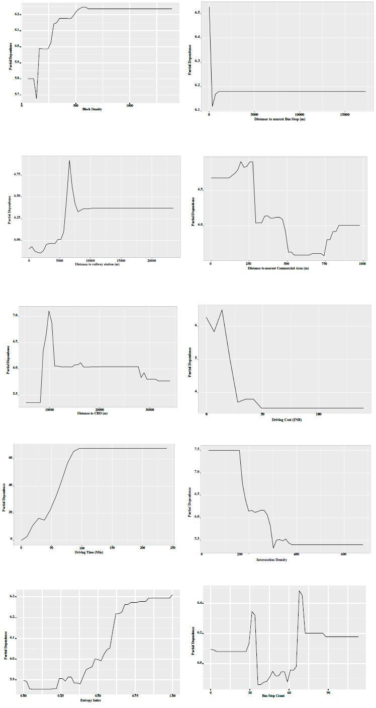
The nonlinear correlations between the built environment and driving travel distance [52].
The plots reveal non-linear relationships between various built environment variables and driving distance in Mumbai, India. These non-linear patterns suggest the complex nature of the relationships between urban form, transportation infrastructure, and driving behavior. While our partial dependence plots examine each built environ- ment factor separately, the varying effects observed across different ranges of each factor indicate that their influences on driving distance are not straightforward. This complexity suggests that these factors likely interact in ways that affect driving behavior, though our current analysis does not directly measure these interactions [7, 73].
For block density, moderate increases sharply raise driving distances due to higher intersection frequency and congestion, supporting previous findings [55]. Beyond 300 blocks per km2, driving distance plateau is around 600 blocks per km2, possibly due to a shift to alternative transport modes or mixed land use [74]. Regarding the distance to the nearest bus stop, driving drops sharply as the distance increases up to 500 meters, indicating that proximity to bus stops discourages car use due to the convenience of public transit. Beyond 500 meters, this effect levels off, suggesting other factors like personal preferences influence driving behavior. For the distance to the nearest commercial area, driving peaks around 75 meters, indicating a transition zone where destinations are close but still require transport. Within 150 meters, driving drops sharply as people prefer other modes due to proximity. Beyond 150 meters, driving rises again, peaking at 225 meters, before gradually declining further out.
Examining the distance to the nearest railway station, driving peaks sharply at around 5,000 meters, indicating high reliance on private vehicles in areas with limited access to railway stations. As the distance decreases from this peak, driving propensity drops notably until around 10,000 meters. Trip cost shows that the propensity for driving peaks at low costs, indicating affordability's significant influence. As driving costs increase, this propensity drops sharply, suggesting sensitivity to cost increases and a shift towards alternative modes. For trip duration, there is a strong, positive relationship between driving time and driving distance. As driving time increases from 0 to around 90 minutes, driving distance rises steadily and sharply. Beyond 90 minutes, driving distances stabilize, aligning with the notion of a travel time budget [65].
Intersection density shows that at lower densities (up to around 200 intersections per km2), driving declines steeply. As density increases beyond 200 intersections per km2, driving rises sharply, peaking at around 400 intersections per km2. Beyond this peak, driving declines, likely due to congestion and complexity in very high-density areas. The entropy index, measuring mixed land use, shows that as it increases from 0.25 to 0.5, driving distances rise gradually. Beyond an entropy index of 0.5, driving distances increase sharply and plateau at an entropy index of 1.0, indicating higher land use diversity correlates with greater driving distances.
Regarding bus stop count, driving distances initially decline with a low number of bus stops, then rise as the count reaches around 30. However, beyond 40-70 bus stops, driving distances sharply decline, indicating numerous bus stops can create congestion or enhance public transport accessibility, reducing the need for driving. Finally, examining the distance to the CBD, there is a sharp peak in driving around 10,000 meters from the CBD, indicating high reliance on cars in suburban or exurban areas with limited public transportation. Closer to the urban core (within 20,000 meters), the propensity for driving drops significantly. These non-linear relationships highlight the need to consider spatial variations and proximity to urban centers in transportation policy and urban development strategies. The observed patterns underscore the importance of the built environment in shaping driving decisions, aligning with the perspectives of scholars who emphasize the role of urban form and infrastructure in influencing travel behavior (Ewing & Cervero, 2001; Gim, 2013) while also acknowledging the interplay with demographic and individual characteristics (X. Cao & Fan, 2012; Stead, 2001).
CONCLUSION
This study provides a comprehensive analysis of the impact of built environment factors on travel behavior in the rapidly urbanizing context of Mumbai, India. By employing Gradient Boosting Decision Trees (GBDT), we capture the complex, non-linear dynamics between the built environment and driving distances. The findings reveal that built environment factors, particularly trip time, distance to commercial areas, and intersection density, significantly influence travel behavior, with socio-demographic factors having a comparatively lesser impact. These insights challenge the traditional view that demographic factors are the primary determinants of travel behavior and highlight the importance of urban form in shaping mobility patterns.
This research also identifies critical thresholds and effective ranges for built environment parameters significantly impacting driving distances. For instance, driving distances increase sharply with higher block density but stabilize beyond a certain point, indicating the influence of congestion and mixed land use. Similarly, proximity to bus stops and commercial areas significantly reduces driving distances, emphasizing the importance of accessible public transportation and amenities in promoting sustainable travel behavior. In response to the comment regarding the focus on driving travel distances, we also recognize the importance of analyzing active travel modes and public transport. While this study primarily focuses on driving, it lays the foundation for future research to explore how the built environment influences other modes of travel, particularly in the context of promoting sustainable mobility solutions in developing countries.
Our results have important implications for urban planning and transportation policies in developing regions. Policymakers should consider these non-linear relation- ships and thresholds when designing urban environments to encourage sustainable mobility. By optimizing factors, such as density, accessibility, and connectivity, cities can reduce reliance on private vehicles and promote active travel and public transport use. However, it is important to acknowledge that the findings are specific to Mumbai and may not be directly applicable to other cities with different urban dynamics. Future research should extend this analysis to other rapidly urbanizing cities in developing countries to validate and refine the conclusions drawn here. In conclusion, this study contributes to the growing body of literature on the built environment and travel behavior, particularly in the context of rapidly developing regions. The insights gained from this research can inform data-driven urban planning and transportation policies that promote sustainable mobility solutions tailored to the unique challenges of cities like Mumbai.
POLICY IMPLICATIONS AND LIMITATIONS
The results of this study suggest important policy recommendations for urban planning and transportation in rapidly urbanizing developing countries like India. To reduce dependence on private vehicles, policies should focus on improving accessibility and connectivity by expanding comprehensive public transport systems and enhancing last-mile solutions, such as feeder buses, bike-sharing schemes, and pedestrian infrastructure [6, 75]. Promoting mixed-use development within urban areas can encourage the use of public transportation and active travel modes, as it reduces travel distances and supports more sustainable travel behaviors [15, 63] Urban density should be carefully managed to ensure it decreases travel distances without leading to congestion and a decrease in quality of life [29]. There is a crucial need for investment in active travel infrastructure, such as walking and cycling pathways, to promote healthier and more sustainable travel options [4]. Tailoring urban planning strategies to different travel purposes, such as enhancing public transport facilities for daily commutes and developing recreational trails for leisure activities, is essential (Ding, Cao, & Wang, 2018). Employing advanced analytical techniques, including machine learning, in data-driven urban planning can provide detailed insights into travel behavior and support the design of effective interventions [7]. Policy measures should also encourage sustainable transportation modes over private car usage through initiatives like congestion pricing and incentives for public transport use [28].
Nevertheless, this study is constrained by the use of existing datasets, which may have limitations regarding sample size, representativeness, and data quality, under- lining the need for robust data to accurately capture the dynamics of travel behavior [76]. The reliance on self-reported data could introduce biases [77]. Moreover, our findings may be specific to the context of the study, echoing concerns from previous research about the challenges of applying models developed in one context to another, particularly from developed to developing countries [78]. Additionally, the study aggregates travel behavior by mode and does not explore variations within these categories.
RECOMMENDATIONS FOR FUTURE RESEARCH
Future research should aim to overcome these limitations by carrying out longitudinal studies that monitor changes in active travel behavior over time and evaluate the effects of specific interventions, as suggested for establishing causal links [79]. Employing qualitative methods, such as interviews or focus groups, can yield deeper insights into the incentives and obstacles to active travel among various demographic groups [77]. Additionally, it is essential to explore the effectiveness of targeted interventions in the built environment, such as infrastructure upgrades and zoning policies, in reducing dependence on motorized transportation to better inform policy decisions [80].
AUTHORS’ CONTRIBUTIONS
A.S.: The study concept and design were contributed; V. P.: Validation was provided.
LIST OF ABBREVIATIONS
| GBDT | = Gradient Boosting Decision Trees |
| MMR | = Mumbai Metropolitan Region |
| VMT | = Vehicle miles traveled |
| VHT | = Vehicle hours traveled |
| BE | = Built environment |
| CBD | = Central Business District |

