All published articles of this journal are available on ScienceDirect.
Travel Time Prediction Using Machine Learning Algorithms: Focusing on k-NN, LSTM, and Transformer
Abstract
Background
Travel time prediction is fundamentally important in advanced traveler information systems. Particularly, in the Dedicated Short-Range Communications (DSRC) traffic information system targeted by this study, travel times are obtained after vehicles terminate trips on the route, indicating that a time-lag phenomenon is inevitable. Therefore, travel time prediction is even more emphasized in DSRC systems. With advances in artificial intelligence technologies, many new machine learning algorithms have recently been introduced.
Methods
In this study, three machine learning algorithms-k-Nearest Neighbor (k-NN), Long Short-Term Memory (LSTM), and Transformer were applied to predict travel times collected on a DSRC-equipped national highway. Travel time outliers caused by entry and exit maneuvers at intersections were filtered using a robust outlier treatment algorithm.
Results
From applying the prediction algorithms, errors of 12.4%, 11.7%, and 10.3% were revealed for k-NN, LSTM, and Transformer, respectively. To identify the statistical significance of the differences in prediction performance, paired t-tests were performed. Consequently, all the differences between the algorithms were proven to be statistically significant. The differences in performance were found to be generally more significant under congested conditions compared to uncongested conditions.
Conclusion
The enhanced reliability of real-time travel time information can increase the effectiveness of DSRC traffic information systems by encouraging drivers to divert from congested routes or adjust their trip schedules to less congested periods.
1. INTRODUCTION
The Advanced Traveler Information System (ATIS) offers road users real-time travel time/speed information [1]. Drivers who receive this information can help mitigate road congestion by avoiding congested areas or adjusting their departure times. Even in the absence of detour routes, drivers informed about upcoming traffic conditions can better estimate their arrival times at the destination, thereby minimizing losses associated with schedule delays [2].
The detection system for ATIS is broadly divided into two types: point detection systems and section detection systems. Point detectors collect traffic flow data from a specific point on the road to calculate the travel time for a section, while section detectors measure the actual time it takes for a vehicle to traverse a section. Point detectors offer the advantage of real-time information, but errors may occur when estimating section travel time based on point speeds. Section detectors, on the other hand, capture the actual travel time experienced by the vehicle, but since the information is collected based on the arrival time, it inevitably results in a time delay. To mitigate this time delay issue, the application of appropriate prediction techniques is essential [3]. This study proposes a methodology for predicting travel time using data collected from Dedicated Short-Range Communications (DSRC) probes on a signalized suburban arterial. DSRC is a representative section detection system in Korea, which collects section travel time by utilizing the identification (ID) numbers of vehicles equipped with DSRC transponders. As of 2021, 270 DSRC receivers have been installed on suburban highways [4].
There have been numerous studies on travel time prediction, but with recent advancements in Artificial Intelligence (AI) technology, new algorithms have emerged. Initially designed for fields such as image recognition and natural language processing, these AI algorithms are now being applied to a wide range of areas, including weather forecasting and stock market analysis. In this study, we predict travel time using both the traditionally employed machine learning algorithm, k-Nearest Neighbor (k-NN), and more recently developed AI algorithms, such as Long Short-Term Memory (LSTM) and Transformer. We then compared and analyzed the performance of these algorithms. The section analyzed in this study currently employs the k-NN algorithm for travel time forecasting. However, to improve the reliability of the predicted travel times, newly developed AI algorithms are being considered. Therefore, the results of this study, which compare and analyze the current algorithm (k-NN) with newer algorithms (LSTM, Transformer), can serve as valuable reference material for system enhancement.
2. PREVIOUS STUDIES
Traditionally, k-NN models have been widely employed for travel time prediction. Kim et al. predicted travel time for the section between Anseong JC and Osan IC using freeway DSRC data. They employed a k-NN model and random numbers for the prediction, achieving an error rate of 4%, demonstrating excellent results. When random numbers were excluded from the historical data pattern, the error rate rose to 18.98%, indicating that the pattern database is a critical factor for prediction accuracy [5]. Lim et al. also used DSRC data from national highways and the k-NN algorithm to predict travel times [6]. Han et al. conducted a study to evaluate the reliability of travel times between toll booths using DSRC data collected from highways [7]. Jang et al. developed a k-NN model to predict fire truck travel times to ensure fire suppression within the golden time during fire incidents. They used 17 independent variables in their analysis and confirmed that fire truck travel times varied depending on land use patterns [8]. Lee et al. proposed a route-based travel time prediction methodology for freeways to overcome the limitations of existing link-based prediction methods. Using a machine learning-based self-organizing map clustering algorithm, and they found that the route-based travel time prediction reduced errors compared to the traditional k-NN model, particularly noting a significant reduction in travel time errors on the Jungbunaeryuk Expressway section of the Seoul-Daegu route [9]. Finally, Park et al. conducted a study on DSRC travel time prediction, addressing the time lag that inevitably occurs when data is collected based on the arrival time. Applying the k-NN algorithm to DSRC data collected from National Highways, they found that the error rate for the analyzed sections ranged from 1.0% to 14.0% [10].
Recently, newly developed AI algorithms have been garnering much attention for travel time prediction. Duan et al. applied the LSTM methodology to predict travel time using data collected from highways in the UK. The prediction results showed an average error rate of 7.0% [11]. Zhang et al. proposed an LSTM-based seq2seq model for short-term travel time prediction and demonstrated superior performance compared to existing methods [12]. Ho et al. proposed a machine learning-based prediction methodology using travel time data collected in Taiwan. The model predicted travel time for one hour ahead to enhance user utility, and the hybrid model employed XGBoost and a fully connected network. The application of the developed model demonstrated superior performance in travel time prediction compared to existing models [13]. Liu et al. predicted bus travel times using vehicle location data collected from buses to forecast urban bus arrival times. The prediction methodology applied a Kalman filter-LSTM model. Since the number of buses is relatively small compared to regular vehicles, the Kalman filter was used to remove noise in individual bus travel times, and the LSTM model was applied for prediction. The results showed that the developed model outperformed existing models [14]. Qiu et al. utilized the random forest algorithm to forecast freeway travel times based on data gathered from probe vehicles. The effectiveness of the proposed prediction methods was rigorously assessed through the calculation of mean absolute percentage errors. These errors were computed across various observation segments, with the prediction horizons varying between 15 and 60 minutes [15].
Several studies have explored the use of machine learning algorithms to predict bus arrival times. Petersen et al. employed an LSTM network to forecast bus travel times using data from Copenhagen. Their model, which incorporated spatiotemporal correlation analysis, demonstrated a marked improvement in prediction accuracy over traditional methods [16]. Comi et al. investigated bus travel time series using seasonal and trend decomposition with Loess, revealing the importance of designing timetables based on the time of day and day of the week, consistent with findings from other global cities [17]. Chen et al. introduced a Bayesian probabilistic model for predicting bus travel times and estimated arrivals, showing that this approach outperformed baseline models by better accounting for bus-to-bus interactions in both predictive averages and distributions [18].
As reviewed, numerous studies have been conducted on travel time prediction to address the time lag phenomenon in section detection systems and provide valuable information for users making route choices. In Korea, traditional statistical and machine learning models have predominantly been employed. Consequently, this study carried out travel time predictions using both the conventional machine learning algorithm (k-NN) and recently developed models (LSTM and Transformer), followed by comprehensive analyses of their performances.
3. METHOD
3.1. k-nearest Neighbor
The k-NN algorithm is a machine learning technique that has traditionally been widely used for travel time prediction. It predicts travel time by selecting the k past travel times that exhibit the most similar patterns to the current collected travel time and averaging them. The steps of the algorithm are as follows [19].
1. k value determination: Decide the number of neighbors (k) from the historical travel times that have similar patterns to the current travel time.
2. Distance calculation: The distance used to search for the number of neighbors with patterns similar to the current travel time among the historical travel times is typically the Euclidean distance (Eq. 1).
 |
(1) |
where d(p, q) = distance between p (present travel time) and q (historical travel time)
3. k neighbors search: Search for the k neighbors from the historical travel times that are most similar to the current travel time.
4. Travel time prediction: Predict travel time by averaging the k neighbors.
The k-NN algorithm is widely used due to its simplicity and strong predictive performance, as evidenced by its frequent application in numerous studies. However, one of its key limitations is the high computational load, as it requires searching for k neighbors in the historical travel time database each time new travel time data is collected, resulting in reduced real-time efficiency.
3.2. Long Short-term Memory
LSTM, a type of Recurrent Neural Network (RNN), addresses the vanishing gradient problem, which is a limitation of traditional RNN models, and demonstrates excellent performance in time series data prediction. By integrating memory cells and gating mechanisms, LSTM controls the flow of information in long-term time series data, minimizing the effects of memory loss. The LSTM network consists of a structure with three gates: forget gate, input gate, and output gate [20].
1. Forget gate (ft): The gate that determines the forgetting rate of the previous cell state (Eq. 2).
 |
(2) |
where σ = activation function, Wf = weight matrix for the forget gate, ht-1 = hidden state of previous step, xt = input at time t, and bf = error term of the forget gate
2. Input gate (it): The gate that determines the new information to be added to the current cell. The similarity between input data is calculated using the Euclidean distance (Eq. 1).
3. Output gate (ot): The gate that controls the output of the cell state (Eq. 3).
 |
(3) |
where Wo = weight matrix for the output gate and bo = error term of the output gate.
3.3. Transformer
The transformer algorithm, first introduced in 2017, serves as the foundation for large natural language processing models. It is highly effective in processing long-term data, and more recently, it has been applied in building time series prediction models in various fields, such as weather forecasting and stock market analysis. Transformers use the attention mechanism (Eqs. 4 and 5) to analyze the correlation between the input (Encoder) and output (Decoder), which has been shown to outperform traditional models in terms of concurrency and learning efficiency [21].
 |
(4) |
where X = input matrix, Q = query, K = key, V = value, and WQ . WK . WV = learned weight mateix.
 |
(5) |
where dk = magnitude of key (index) vector and KT = transpose matrix of K.
Since the Transformer does not perform recurrent or convolutional operations, the order of the time series data must be encoded. This is achieved by using sine and cosine functions, as shown in Eqs. (6 and 7), to input positional (order) information. By employing sine and cosine functions, the position of the data can be set continuously and smoothly.
 |
(6) |
 |
(7) |
where pos = position (order) of time series data, i = dimension of positional encoding, and dmodel = dimension of positional encoding.
4. DATA
4.1. Experiment Section
The travel time data were collected using two DSRC receivers installed on National Highway 38 in Pyeongtaek City in Korea. As shown in Fig. (1), the data collection section covers 4 kilometers and contains a total of six signalized intersections. Although the speed limit is 80 km/h, due to the dense placement of traffic signals, the average speed during non-congestion periods was around 50 to 60 km/h. The Pyeongtaek Industrial Complex is located near this section, leading to congestion during weekday morning rush hours. No congestion occurs on weekends when there is no commuting traffic, so data collection was conducted on weekdays in January 2013, when morning congestion was observed. Since travel times remain relatively consistent throughout the day on congestion-free weekends, predictive algorithms were not applied, and weekend data were excluded from collection and analysis (Fig. 2).

Study section.
Outlier removal process.
Probe travel times: (a) raw data and (b) outlier-filtered data.
4.2. Outlier Treatment
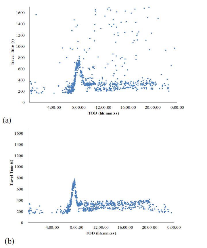
The target section exhibits the characteristics of a typical interrupted facility. Due to significant traffic inflows and outflows at intersections, shops, and gas stations within the section, a large number of outliers were collected, as shown in Fig. (3a). These outliers were processed using an algorithm developed for outlier removal, as described in Eqs. (8-11). The distribution of individual travel times, with the outliers removed, is shown in Fig. (3b).
 |
(8) |
 |
(9) |
 |
(10) |
 |
(11) |
where
N = number of travel times,
TAB(t) = average of valid travel times from A to B at time t,
SAB(t) = set of valid travel times from A to B at time t,
tA(B),i(j,k)(t) = detection time of vehicle i (j, or m) at point A or B,
tw = aggregation interval (5 min), and
zm = z-score (4.45) at 99.9% confidence interval for median.
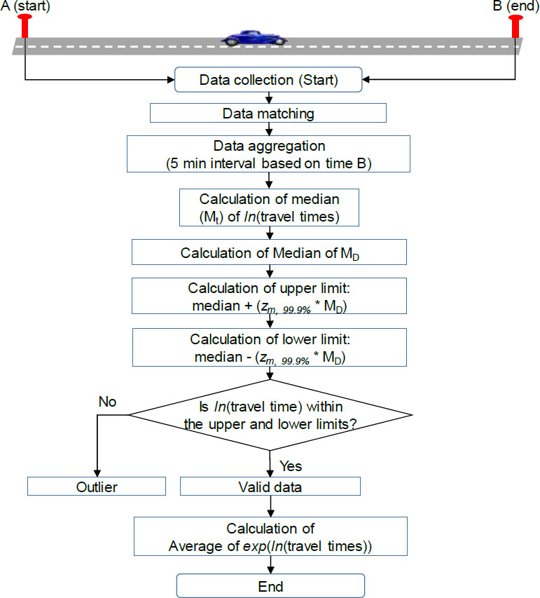
The outlier filtering algorithm removes aberrant data that fall outside the calculated confidence interval, which is determined based on the median within an aggregation interval (Eqs. 9-11). Subsequently, an average travel time is computed using the filtered data (Eq. 1). The algorithm's novelty lies in its use of the median and log-normal distribution, specifically tailored to the travel time characteristics of signalized arterials, as demonstrated in a previous study [22], where travel times were found to follow a log-normal distribution. Additionally, the modified z-score (z-score / 0.6745) was used to adjust the confidence interval for the median [23]. The step-by-step process of the filtering algorithm is depicted in Fig. (2).
4.3. Filtered Travel Time Data
The distribution of filtered travel times in 5-minute aggregation intervals is presented in Fig. (4). Recurrent congestion occurred between 8:00 and 8:30 AM. Although increases in travel time were observed in the afternoon, they were relatively modest compared to the morning peak periods. The total number of data points for the 5-minute aggregation interval was 5,181, with data collected over approximately 18 days. As shown in Table 1, the average travel time for the study section was 283 seconds, with a standard deviation of 106 seconds, a minimum of 130 seconds, and a maximum of 1,193 seconds. The maximum travel time was nearly five times the average, indicating significant congestion during the morning peak hours.
5. TRAVEL TIME PREDICTION
A total of 5,181 travel time data points were divided into training (70%) and testing (30%) sets. Z-score scaling was applied to expedite convergence and improve model performance. Travel time predictions were set 30 minutes ahead, considering that morning congestion typically lasts for approximately 30 minutes. Although the prediction intervals varied from 10 to 60 minutes, no significant differences in predictive performance were observed. The LSTM and Transformer networks were developed using the TensorFlow Keras framework.

Filtered travel time data in 5-minute intervals.
| Statistic | Travel Time (sec) |
|---|---|
| Count | 5,181 |
| Mean | 283 |
| Standard deviation | 106 |
| Minimum | 130 |
| Maximum | 1,193 |
5.1. k-nearest Neighbor
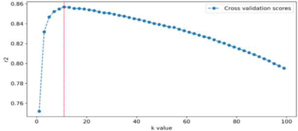
The k-NN algorithm predicts travel time by searching for k historical travel time patterns similar to the current travel time pattern and calculating their average. Therefore, determining the optimal k value that maximizes prediction performance is crucial. Fig. (5) illustrates the process of identifying the optimal k value. After exploring k values from 1 to 100, the best performance was observed at k = 11. In this study, the travel time patterns used for the optimal k value search were based on 30-minute intervals (6 travel time values in 5-minute aggregation intervals).
k-NN performance by number of k value.

Comparison of actual and predicted travel time (k-NN).
| Parameter | Search Grid | Optimal |
|---|---|---|
| Number of neighbors | [1 – 100] | 11 |
| Distance metric | [Manhattan, Euclidean, Minkowski] | Euclidean |
When searching for the optimal k value, the similarity between historical travel time patterns is typically assessed using distance metrics such as Manhattan, Euclidean, and Minkowski distances. In this study, Euclidean distance, which demonstrated the best prediction performance among the three metrics, as shown in Table 2, was used as the similarity evaluation metric. A review of previous studies in Chapter 2 also revealed that Euclidean distance was the most commonly used metric.
Fig. (6) illustrates the distribution of predicted travel times compared to the actual travel time distribution. Overall, the predicted travel times exhibited a pattern similar to the actual travel times; however, during the morning peak hours, the predicted travel times were lower than the actual values. Given the importance of accurate travel time information during periods of severe congestion, this result is somewhat unsatisfactory.
5.2. Long Short-term Memory
LSTM is a recurrent neural network model specialized for time-series data prediction, where the setting of the time-series data cycle is critical. In this study, considering that travel times exhibit daily periodicity, the cycle was set to 288 (5-minute aggregation intervals * 24 hours). Since vehicle traffic is closely related to human activity patterns, it is considered reasonable to set the cycle on a daily basis.
The optimal parameters of the LSTM model were obtained using the grid search methodology proposed by Abbasimehr et al. [24], as shown in Table 3. Mean Square Error (MSE) was employed as the loss function, and Adaptive Moment Estimation (Adam) as the optimizer. While the number of epochs was set to 100 with an early stopping callback (patience of 5), the model was optimized at the 69th epoch. It was observed that increasing the number of hidden nodes beyond 128 resulted in overfitting, leading to a decline in model performance.
Fig. (7) illustrates the learning process of the developed LSTM model. As the model was optimized at the 69th epoch, the horizontal axis is displayed up to 69 epochs. It can be observed that the rate of error reduction significantly decreases after the 20th epoch. Fig. (8) shows the distribution of predicted versus actual travel times. While the prediction performance during peak hours, a known limitation of the k-NN algorithm, was satisfactory, the discrepancy between predicted and actual travel times during non-peak hours was relatively large, highlighting the need for further investigation into more effective prediction models.
| Parameter | Search Grid | Optimal |
|---|---|---|
| Number of hidden node | [64, 128, 256] | 128 |
| Activation function | [Sigmoid, Tanh] | Tanh (hyperbolic tangent) |
| Window size | [144, 288, 576] | 288 (24 hours) |
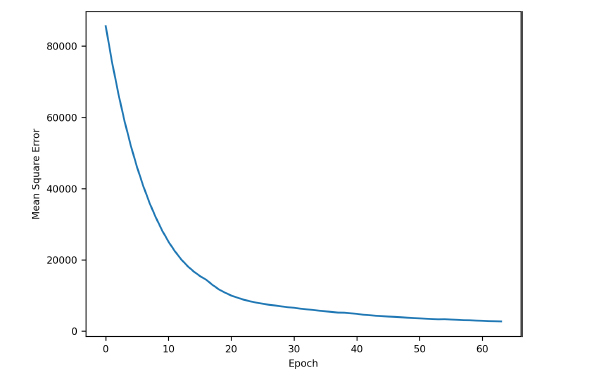
Learning process (LSTM).

Comparison of actual and predicted travel time (LSTM).
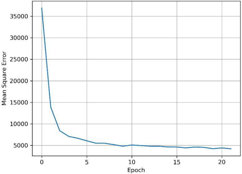
Learning process (transformer).
| Parameter | Optimal |
|---|---|
| head_size | 256 |
| num_heads, ff_dim, num_transformer_blocks | 4 |
| mlp_units | 128 |
| mlp_dropout | 0.2 |
| dropout | 0.1 |
5.3. Transformer
The Transformer model was developed to address the limitations of the LSTM model and therefore, shares similar characteristics. Accordingly, the cycle was set to 288, as with the LSTM model. The Transformer parameters were optimized using the weight initialization methodology proposed by Huang et al. [25], as shown in Table 4. The loss function, optimizer, batch size, and epochs were set the same as in the LSTM algorithm, and the model was optimized at the 22nd epoch.
Fig. (9) shows the learning process of the constructed Transformer model. Since the model was optimized at the 22nd epoch, the horizontal axis is displayed up to 22 epochs. Unlike the LSTM model, the Transformer model shows a sharp reduction in the error rate after just 3 epochs. Fig. (10) demonstrates the distribution of predicted versus actual travel times. Compared to the k-NN and LSTM models, the Transformer model exhibited superior performance during both peak and non-peak hours.
6. RESULTS & DISCUSSION
To quantitatively evaluate the performance of the developed models, Mean Absolute Error (MAE), Root Mean Square Error (RMSE), and Mean Absolute Percent Error (MAPE) were used as evaluation metrics, as shown in Eqs. (12-14). MAE is the average of the absolute errors and is easy to interpret, while RMSE always has a larger value than MAE since it is calculated by dividing the square of the errors. According to Hodson [26], MAE is advantageous when errors follow a normal distribution, whereas RMSE is more suitable when errors follow a Laplace distribution. Due to the distinct characteristics of these metrics, it is common practice to use both in the evaluation of regression models. MAPE expresses MAE as a percentage, making it easier for users to intuitively understand.
 |
(12) |
 |
(13) |
 |
(14) |
where y = observed value,  = predicted value, and n = number of sample.
As shown in Table 5, the Transformer model outperformed all others across all evaluation metrics, followed by the LSTM model. The k-NN model, which was primarily used for travel time prediction before the development of deep learning models, showed the lowest performance across all metrics. However, the performance difference was not substantial, ranging between 1 to 2%. To test the statistical significance of these performance differences, a paired t-test was conducted. As indicated in Table 6, the p-values for the performance differences between the three models exhibited lower than 0.05, proving that the performance differences are statistically significant at a 95% confidence level. For brevity, only the MAPE results of the t-test are reported, but similar results were observed for the other two metrics.

Comparison of actual and predicted travel time (transformer).
| Algorithm | k-NN | LSTM | Transformer |
|---|---|---|---|
| MAE (sec) | 31.8 | 29.3 | 27.6 |
| RMSE (sec) | 41.2 | 38.0 | 37.3 |
| MAPE (%) | 12.4 | 11.7 | 10.3 |
| Statistic | k-NN | LSTM | LSTM | Transformer | k-NN | Transformer |
|---|---|---|---|---|---|---|
| Mean | 12.4 | 11.7 | 11.7 | 10.3 | 12.4 | 10.3 |
| Variance | 95.2 | 117.9 | 117.9 | 83.7 | 95.2 | 83.7 |
| t-value | 2.53 | 3.18 | 5.26 | |||
| p-value (one-sided) | 0.0058 | 0.0007 | 8.59E-8 | |||
| Number of sample | 1137 | |||||
To conduct a detailed performance analysis, the results were classified based on traffic flow conditions. A threshold of 300 seconds was chosen, considering the flow conditions of the experimental section. Table 7 presents the t-test analysis for cases exceeding 300 seconds, while Table 8 shows the analysis for cases equal to or less than 300 seconds, and Fig. (11) illustrates the MAPE differences between the two traffic conditions. Overall, the performance differences were more pronounced during congestion compared to non-congested periods. Although the performance gap between the LSTM and Transformer models was slightly larger during non-congested periods, the difference was not substantial compared to other cases. This likely stems from the increased LSTM error rates during off-peak hours, as previously mentioned. In all cases, except for the performance difference between k-NN and LSTM during non-congested periods, the performance differences were statistically significant.
| Statistic | k-NN | LSTM | LSTM | Transformer | k-NN | Transformer |
|---|---|---|---|---|---|---|
| Mean | 12.0 | 10.5 | 10.5 | 9.3 | 12.0 | 9.3 |
| Variance | 101.4 | 88.0 | 88.0 | 51.9 | 101.4 | 51.9 |
| t-value | 3.39 | 2.06 | 4.45 | |||
| p-value (one-sided) | 0.0004 | 0.02 | 5.52E-6 | |||
| Number of sample | 388 | |||||
| Statistic | k-NN | LSTM | LSTM | Transformer | k-NN | Transformer |
|---|---|---|---|---|---|---|
| Mean | 12.5 | 12.2 | 12.2 | 10.8 | 12.5 | 10.8 |
| Variance | 92.1 | 132.6 | 132.6 | 99.6 | 92.1 | 99.6 |
| t-value | 0.87 | 2.51 | 3.42 | |||
| p-value (one-sided) | 0.19 | 0.006 | 0.0003 | |||
| Number of sample | 749 | |||||
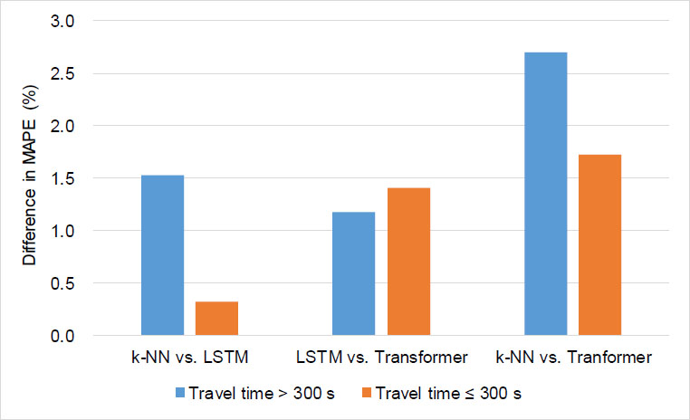
Performance differences between models based on flow conditions.
CONCLUSION AND FUTURE STUDIES
The reliability of real-time travel time information is a crucial factor in evaluating the effectiveness of Advanced Traveler Information Systems (ATIS). Over the past 30 years, numerous studies have focused on ensuring the reliability of travel time data. In section detection systems such as DSRC, generating predicted travel time information to mitigate time delay effects is particularly important. In this study, we utilized the LSTM and Transformer algorithms, both known for their strengths in time-series data prediction and their emergence alongside advances in AI technologies, to predict travel times on a signalized suburban arterial. For comparison, the current method (k-NN algorithm) was also applied. Due to the nature of signalized arterials, characterized by interrupted traffic flow and numerous outliers from intersection entries and exits, a previously developed DSRC outlier removal algorithm was used to effectively filter the aberrant data.
The data used for prediction was collected in January 2013 on weekdays using a pair of DSRC transponders installed at 4 km spacing. The study section is located near the Pyeongtaek industrial complex, where recurring congestion occurs between 8:00 and 8:30 AM on weekdays. During congestion, travel times increased by approximately five times compared to non-congested periods. Consequently, this section was identified as a critical area for providing travel time predictions to encourage the use of alternative routes or adjustments in departure times.
The application of the prediction algorithms showed that the Transformer algorithm performed the best in all cases. The k-NN algorithm underestimated travel times during peak hours, while the LSTM algorithm exhibited increased errors during the early morning hours when traffic volume was the lowest. The prediction errors for each model were 12.4%, 11.7%, and 10.3% for k-NN, LSTM, and Transformer, respectively. A statistical significance test on the prediction errors revealed that, at a 95% confidence level, the performance differences between the models were significant.
An analysis of performance differences by traffic conditions indicated that the differences between models were generally more pronounced during congested periods than during non-congested periods. Given that travel time prediction is particularly crucial during congestion, it is considered that applying the LSTM and Transformer algorithms is more advantageous than the conventional k-NN algorithm.
This study analyzed the predictive performance of various algorithms using data collected over approximately one month. To ensure the generalizability and applicability of the results, further research should be conducted on segments that exhibit more diverse traffic patterns.
AUTHORS’ CONTRIBUTION
The author confirms sole responsibility for the following: study conception and design, data collection, analysis and interpretation of results, and manuscript preparation.
LIST OF ABBREVIATIONS
| DSRC | = Dedicated Short-Range Communications |
| LSTM | = Long Short-Term Memory |
| ATIS | = Advanced Traveler Information System |
| AI | = Artificial Intelligence |
| RNN | = Recurrent Neural Network |

