All published articles of this journal are available on ScienceDirect.

A Game Theory Approach to Trip Distribution Model: Game Distribution Model
Abstract
Introduction
In Transport planning, the four-step travel demand model is one of the most popular macro scale planning tools since the 1970s. The second step of this traditional model, i.e., trip distribution, plays an essential role in the model and at the same time, it is the most controversial step.
Methods
Various alternative approaches are available in the literature for modelling trip distribution, such as the Gravity Model, intervening opportunities model, logit models etc. However, none of these models is universally accepted. Although the gravity model is the most common and well-known trip distribution model, it is often subject to the same criticisms as other alternative models. In this study, the trip distribution step of the four-step model is designed as a rational game to replicate preferences in a more realistic way. The usual assumption in the traditional distribution model is that decision-makers are influenced by only origin/destination-based travel attributes and/or impedance of the trip to the destination. However, other probable destination circumstances are not included in this procedure. In order to incorporate the actual determinants of trip making, Traffic Analysis Zones (TAZ) are considered to be gamers in the proposed model, and the generalized trip cost was considered to be the cost of gamers. Each TAZ has a utility that attracts individuals from other TAZs. Trips are distributed by comparing the utility of a TAZ with the associated cost. Empirical verification of the model is performed by using the household survey data for Eskişehir/Turkey.
Results
The evaluation was performed with different goodness of fit statistics for 5 different structured O/D matrices representing various demand settings. The results indicate that the proposed model demonstrates strong performance according to selected micro- and macro-level goodness-of-fit statistics, with all R2 values exceeding 0.80.
Conclusion
When compared to the classic Gravity Model, these goodness-of-fit measures yield better results in general.
1. INTRODUCTION
People travel to fulfill various activities, and this need directly arises from activity demand, with travel remaining the essential link for achieving these goals. Transportation planning aims to develop models that represent the real world and simulate travel patterns with measurable elements. The aim of developing such models is to understand the present dynamics and make forecasts for the future in order to detect, locate, and solve existing and future problems in transportation systems. These problems often harm not only travelers but also the community through negative impacts, such as waste of fuel, loss of time, and environmental pollution. Interventions that will either affect the supply (road widening, etc.) or the demand (public transport incentives, congestion pricing, etc.) are recommended for the solution of the problems identified with these models. The trips are tried to be aggregated in the widely used transportation planning models, although each trip is the choice of an individual. Recent studies have shown that models that take individual choices and their underlying factors with disaggregated data into account can yield more accurate results.
The modelling field is dominated by the approach known as the four-step travel demand model. In this model, trips are evaluated on a macro scale, and aggregated data are used in all steps. It uses generalized features such as population and employment rather than passenger characteristics. Accordingly, this model does not consider the effects of trips on each other. Four-step travel demand model has four steps: trip generation, trip distribution, mode choice, and trip assignment. In the trip generation step, the number of trips that start and end at each of the sub-regions is estimated. These sub-regions are named as Traffic Analysis Zones (TAZ). TAZs are tried to be established in such a way that they contain homogenous users. Trip distribution is the second step of the four-step model and addresses the question of how many trips occur between each TAZ pair. The outputs of trip distribution are origin-destination zonal trip tables (O/D matrices) by purpose. These O/D matrices are split into the travel modes, and a separate matrix for each mode is determined at the mode choice step. The final step in the four-step model is the trip assignment. This step consists of separate highway and transit assignment processes. The highway assignment process determines routes for vehicle trips along the road network, while the transit assignment process determines routes (or options) for using various transit route alternatives.
All steps of the four-step model work together to make the most accurate prediction. The reliability and correctness of each step are critical for the next step and, ultimately, for the success of the model. Especially the second step, trip distribution, has a more important place because both the mode choice and the assignment steps use the O/D matrices determined in this step. Hence, improving trip distribution models is crucial for complete model success.
In the literature, the question of modelling trip distribution has been approached by researchers from different disciplines, such as geographers, economists, and urban planners [1]. The primary purpose of all distribution models is to distribute the total demand from a given origin among the different destinations. The inputs to common trip distribution models include the trip generation outputs and measures of travel impedance between each pair of zones obtained from the transportation network. Additionally, this impedance is usually included in the model as the physical distance or cost of this distance or measured/assigned travel time. While distance is undoubtedly an important factor in trip distribution, it is not the sole determinant. Different models can be produced to improve this situation. In the Intervening Opportunities model, trip making is influenced not only by travel distance but also by accessible opportunities. With advancements in decision-making models, disaggregate models have started to be developed.These models include new dimensions to the analyses including socio-economic factors that could not be addressed before.
In general, travel decisions can be influenced by other passengers' preferences. However, this effect is not considered in classical distribution models. For this reason, this study aims to propose a new model for trip distribution that accounts for preferences. The proposed model will consider trips as a game between TAZs. In this way, the model will not only consider travel impedances between TAZs but also it will incorporate the desire to travel to other TAZs. With the new model's success in expressing actual travel distributions, it will be ensured that the outcome of the classical four-step model will be more useful compared to the previous approaches.
The paper is organized as follows: The next section provides a detailed literature review, including the place of trip distribution in the broader transportation model system and the main approaches used in aggregate trip distribution models. This section also reviews the development of game theory in transportation modelling until today. Section 3 presents the background and details of the proposed model named the Game Distribution Model. In this section, the new model is applied to real-world data and the results are compared with the ones obtained from the traditional model. Section 4 presents the results of the analyses. In the next two sections, the findings and deductions obtained from the model, as well as the limitations of the proposed approach, are discussed and presented.
2. LITERATURE REVIEW
2.1. The Place of Trip Distribution in Transportation Models
By the 1950s, car ownership increased rapidly, and travel modelling became necessary to design future transportation systems considering community needs and expectations. Trip distribution, which is the second step of the travel demand model, is intended to produce the best possible predictions of participant destination choices based on trip generation and attraction information. Two broad approaches are used in travel distribution: aggregate and disaggregate [1]. Aggregate models use data aggregated over a series of geographic sub-regions called TAZs. Together, these zones represent an activity system served by a transportation network, and aggregate models analyze each TAZ’s total number of trips. On the other hand, disaggregate models such as discrete choice models, family, and activity-based models deal with individuals' behaviors and destination choices. These models are generally derived from the notions of utility theory [2].
The first-generation aggregate trip distribution models use growth factors from extensive surveys of origin-destination flows. Growth factor methods may be subdivided into four groups: constant factor method, average factor method, Fratar method, and Furness method. Fratar and Furness are the most popular algorithms [3]. Fratar [4] developed a model that made the factoring of an observed flow matrix. It makes the assumption that the existing trips will increase in proportion to the production and attraction growth factors of TAZs. After the Fratar model, Furness [5] proposes a model which is one of the best known iterative methods that uses two growth factors and two balancing factors. All growth factor methods work regardless of increased supply or changed spatial accessibility that occur due to changes in travel patterns and congestion [6].
In addition to growth factor models, there are synthetic distribution models in the literature. These models attempt to identify the causes of current travel patterns and then assume that these underlying causes will remain the same in the future [3]. The most well-known synthetic distribution model is called the gravity model. The important feature that distinguishes the gravity model from growth factor models is that it models not only according to the demand in the future but also takes into account the concept of the hardship of travelling. The hardship is represented by travel impedances, a feature introduced by the gravity model. The first use of the gravity model occurred in the 1950s, and later, many other aggregate or disaggregate models followed the initial trip distribution techniques.
Disaggregate trip distribution models were developed after significant improvements in the discrete choice modelling technique. These models aim to better predict travel behavior by including variables other than travel time [6]. They calculate the choice probabilities of the individuals or groups of individuals with models such as Multinomial Logit or Nested Logit [7]. Later, more sophisticated models were developed, such as the Mixed Logit [8] and the Activity-Based Approach [9]. There are also some studies examining the use of Artificial Neural Networks in disaggregate trip distribution models [10]. The advantage of these models is that it is possible to introduce different attributes into the decision-making process.
2.2. Main Approaches Used in Aggregate Trip Distribution Models
The primary purpose of this study is to propose a new approach and calculation procedure for aggregate trip distribution models. Therefore, first of all, well-known main aggregate approaches have been explained in this section.
2.2.1. The Gravity Model
The doubly constrained classical gravity model [11] is the best-known and most basic aggregate distribution model. It is named for its similarity to Newton's law of universal gravitation.This model assumes that the number of trips between two locations is related to their populations and decays with an impedance function. The gravity model's inputs include the trip generation outputs (productions and attractions) for each zone and measures of travel impedance between each pair of zones obtained from the transportation network. In addition, socio-economic and area characteristics are sometimes used as inputs as well [12].
Probably the first rigorous use of a gravity model was by Casey in 1955, and the most straightforward formulation of the model has the following functional form [13]:
 |
(1) |
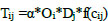
In this model, TijT_{ij}Tij represents the trips between an origin zone i and a destination zone j, while Oi and Dj denote the trip ends produced at i and attracted at j, respectively. The proportionality factor α\alphaα can be replaced by the multiplication of two sets of balancing factors, Ai and Bj, as used in the Furness algorithm [13].
In Eq. (1) f(cij) function represents a generalized function of the travel expense (cost or time) between every pair of zones and has one or more calibration parameters. This function often receives the name ‘deterrence function’ because it represents the disincentive to travel as distance (time) or cost increases. Well-known functional forms are presented in Eqs. (2-4) [14]:
 |
(2) |
 |
(3) |
 |
(4) |
Where β and n are parameters to be calibrated, and cij is the deterrence value.
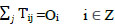
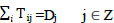
In order for the trip distribution step to be completed, the sum of the trips produced between any origin zone i and all destination zones j ∈ Z (Zones) should be equal to the total trip ends produced at the origin zone. Similarly, the sum of the trips attracted between any origin zone i and all destination zones j ∈ Z should be equal to the total trip ends attracted at the origin zone. These are known as the flow conservation constraints given in Eqs. (5 and 6):
 |
(5) |
 |
(6) |
With its well-known theoretical base, gravity-type spatial interaction models have been the most commonly used aggregate trip distribution models [15]. The gravity model is primarily far easier to estimate, with only one or two parameters in the deterrence function formulas to calibrate and easy application and calibration procedures using various travel modelling software [12].
Despite its widespread use, there are many criticisms of the gravity model. Mainly, it uses an aggregate procedure and does not refer to any explicit individual behavioral theory. Moreover, the model assumes that all information lies in the constraints; it does not consider any perception attributes [1].
2.2.2. Other Approaches
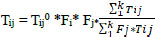
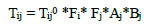
First-generation trip distribution models were used as Growth-factor models. Generally, originating and attracted trip totals are known collectively as an output of the trip generation step. In 1954, A method was introduced by T. J. Fratar to overcome some of the disadvantages of the doubly costraint methods [4]. The multiplication of the existing flow by two growth factors (row and column growth factors from production and attraction values) will result in the future trips originating in zone i being greater than the future forecasts, and so a normalizing expression is introduced [3]. The Fratar formulation is presented in Eq. (7).
 |
(7) |
Tij and Tij0 are the future and observed number of trips between zones i and j. Fi is the row factor from production, Fj is the column factor from attaction. k is the number of total zones.
After the Fratar algorithm, Furness proposed an iterative method in 1965 [5]. In this method, the productions of flows from a zone are first balanced, and then the attractions to a zone are balanced [3]. The equation of this model, in which two growth factors (row factor Fi, column factor Fj) and two balancing factors (Ai and Bj) are used, is given in Eq. (8).
 |
(8) |
The Doubly Constrained Growth Factor Model converges very quickly in most cases and is usually used to model the external to external movements or estimate goods vehicles and freight [16]. This model has two major disadvantages: a zero cell in the matrix remains zero regardless of how many times it is factored. The second is that it is not sensitive to possible changes or enhancements in the transport system.
Another popular approach is the Intervening Opportunities Model developed by Stouffer [17] and refined by Schneider [18] in the Chicago Area Transportation Study. In this model, the distance does not affect the destination choice, playing only the role of a surrogate for the number of intervening opportunities between them [19]. The number of persons going to a given distance is directly proportional to the number of opportunities at that distance and inversely proportional to the number of intervening opportunities.
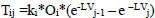
The most widely used form of the intervening opportunities model can be written as shown in Eq. (9) [20]:
 |
(9) |
Tij is the predicted number of trips, ki is a constant or balancing factor, Oi is the total production from origin i, and V is the number of opportunities. Finally, L is a constant probability that a random destination will satisfy the needs of a traveler. According to Ortuzar and Willumsen [13], intervening opportunities model has three main disadvantages. The theoretical basis is less well-known and more complicated than the gravity model. It does not include any practically measured trip deterrence attribute (i.e., cost, etc.) and does not have a suitable software.
2.3. Game Theory
In this section, the background of game theory, which is the main method that the proposed model is built upon, is presented. The basis of game theory is the assumption that an individual who makes choices interacts strategically with other individuals. Players are aware that their decisions affect each other's conditions and make decisions accordingly [21].
John von Neumann (1944) [22] discussed Game Theory, which dates back to Babylon, as an economic study in his book “Game Theory and Economic Behavior”. After that, John Nash's articles on the definition of equilibrium laid the foundations of modern non-cooperative games in the early 1950s [23]. Before the 1970s, studies were carried out by assuming that individuals were fully knowledgeable about all options. By the 1970s, game theory studies were developed considering that information is incomplete and rationality is limited [24].
In economics, all participants aim to maximize their profit. Supply-demand equality, a state in which participants do not tend to change their behavior without any external influence is called the concept of market equilibrium. The most widely used equilibrium theory in strategic structures is the Nash equilibrium, developed by John Nash [23]. In the Nash equilibrium, after both players see the other player's strategy, they will not regret their choice and will continue this strategy if they have a chance to play again [25]. The profit function of each player is given in Eq. (10). In this equation, i represents player i's profit, and s represents the strategies of players.
 |
(10) |
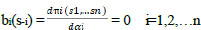
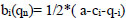
This theory defines decisions as responses to the game. The best response functions are found by taking the derivative of each player's profit function and equalizing it to zero (Eq. 11). With this process, it is aimed to determine the extremum point of response, and this point is named Nash equilibrium. At this point, all players make the decision that they are satisfied with. bi represents the player i's best response, and αi represents player i's action that affects the strategy,
 |
(11) |
The Nash equilibrium is searched for a point where all players determine their decisions, and they do not want to make any changes. On the other hand, Cournot is a model based on quantity competition for participant decisions and was developed long before the concept of Nash equilibrium. Following Nash, Cournot is reinterpreted and has become an integral part of economic analysis [26]. In the Cournot – Nash model, a homogeneous product is produced by n number of companies. The production value of each firm that makes its own profit maximum is determined by the Nash equilibrium.
Profit (π) is found by subtracting the total cost from its total income (Eq. 12). The cost of producing for the i. company is expressed as ci(qi). Where, ci represents unit cost and qi is the production value. Moreover, P(Q) (Q= q1+q2+…qn) represents the market price, which is determined by the demand for goods and the total production amount of the companies. This price has an inverse demand function, if the company's output increases, the price decreases (p= a-Q).
 |
(12) |
Similar to Nash equilibrium, the best response function can be calculated by taking the derivative of the gain according to the strategy action (here, strategy is determined by production value -q). Company i’s best response given Eq. (13).
 |
(13) |
Nash equilibrium is at the intersection of these best response functions.
2.3.1. Game Theory in Transportation
Game theory applications have a wide range of usage areas, from strategic questions on war to animal behavior in competitive situations, to hall games, and even elections. Likewise, it has been used many times in the field of transportation. Zhang et al. [27] classify the game theory studies in transportation into two types: Macro and micro levels. In macro-level transportation games, the analysis focuses on complicated and broad situations involving many players. In micro-level transportation games, the focus is only on a limited circumstance where only a few players exist.
Macro-level games can be between passengers and authorities, between passengers and passengers, or between authorities and authorities. Examples of macro-level games are determining road and parking fees, urban traffic demand, guiding driver reactions, and others [28-50].
The studies conducted at the micro-level usually assessed a part of an overall situation. Consequently, games among authorities can not be included in micro-level games. Traffic Signal Strategies, Plane collisions, and Pedestrian as well as vehicle conflicts are examples of micro-level games [51-64].
3. METHODS
3.1. Proposed Model; Game Distribution Model
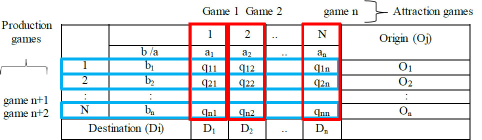
In this study, game theory was used to distribute the production and attraction values obtained from the first step of the classical four-step model. In the proposed methodology, production and attraction values for each TAZ are distributed with a game. Each TAZ is assumed to be a player. Games between TAZ pairs are shown in the form of an O/D matrix in Table 1. All cells in the center of the n x n matrix represent the number of trips (qij) from TAZi (starting point of the trip -origin) to TAZj (the final point - destination). This matrix has n production games and n attraction games.
In every game created for attractions, (shown in red in Table 1), it is assumed that all TAZs traveling to destination TAZ are players aiming to maximize their share of total attraction profit. Players (TAZs) determine the number of trips they can send to optimize their profit, with the number of trips from TAZi to TAZj (qij) being strategy actions for players. The sum of the qij gives the attraction value (∑qij=Q). The profit of the trip from i to j (πij) is calculated by subtracting the total cost (cij) from the total utility (u(Q)). It is shown in Eq. (14).
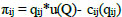 |
(14) |
|
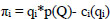
The concept of utility seen in Eq. (14) is created by an analogy with the concept of price in the Cournot – Nash model. Utility motivates passengers to make trips; it is inversely proportional to demand. As the number of trips increases, the utility decreases. Utility depends on the total number of trips, trip origin, and destination characteristics. It is shown in Eq. (15).
 |
(15) |
aj: A parameter that depends on destination TAZ
bi: A parameter that depends on the origin TAZ
u: The utility per trip
Q: Total number of trips (∑qij)
As an advantage, this profit approach allows the use of not only travel cost but also travel time or marginal cost to determine total cost. cij function can be replaced with tij (travel time) or a combination of factors. Even more, other variables, such as the employment or population of the destination TAZ can be added to this equation.
According to the game theory, the best response function is calculated after the profit function is determined. The best response function can be calculated by taking the profit's derivative according to the strategy action (action-the number of trips from TAZi to TAZj (qij)). In the case of n players, there are n best response functions for every attraction (Eq. 16).
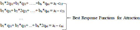 |
(16) |
With the steps and approach mentioned above, n game has been developed for n attraction values, and n best response (bri) has been determined for each attraction (a total of n2 best responses, Eq. (16)).
Production games are developed in the same way and shown in blue in Table 1. TAZs, that have at least one traveler from that TAZ, are players, and they aim to get a share of the total production. The total profit for each TAZ is, again, inversely proportional to demand; if the total number of trips increases, the utility decreases (Eq. 14). Accordingly, n game has been developed for n production values and n best responses (bri) has been determined for each production (a total of n2 best response, Eq. (17)).
 |
(17) |
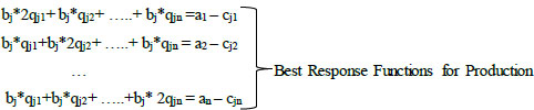
As a result of the construction of attraction and production games, 2*n2 best response functions are formulated. The equilibrium point can be determined by solving these equations together. Additionally, because of the complexity of equations, these best response functions can be designed as a minimization problem, and this problem can be solved using algorithms such as the Generalized Reduced Gradient (GRG) Nonlinear Solving method and others. Game Distribution Model, formulated as a minimization problem, is presented below.
Variables: qij, ai ve bj (n*n+ 2n variable)
Objective: Min ε
ε= (∑ εn)^1/2
b1*2q1i+b2*q2i+ …..+bn *qni - ai-c1i = ε1
b1*q1i+ b2*2q2i+ ….+ bn*qni - ai–c2i = ε2
…
…
bj*qj1+bj*qj2+ …..+bj* 2qjn - an–bn*cjn =εn
Subject to: qji >0, ai>0, bj>0
In the minimization problem mentioned above, due to the nonlinearity of the best response functions, the obtained results are local optimums. Therefore, if there is a preliminary estimate, the minimization problem can yield a better local optimum. In the proposed model, a preliminary estimation does not exist. Thus, an algorithm that accounts for no initial estimates was developed (Fig. 1).
The steps of the algorithm are as follows:
Step 1: Set all variables (qij, ai, bj) to 0 (there is no preliminary estimation.)
Step 2: Solve the minimization problem, then calculate the error (ει) and set vari+1.
Step 3: Compare the recent error (ει) with the previous error (εi-1) to see if any improvement is achieved
Step 4: Any improvement? Update all variables (qij, ai, bj) and error (ει), then go to Step 2.
Step 5: Stop. εi-1 is the final error, and vari are final variables.
3.2. Performance Measures and Goodness of Fit Statistics
The performance and success of the proposed methodology can be assessed by using various measures. In this study, several different goodness-of-fit statistics were selected for performance measurement and model evaluation. Root Mean Squared Error (RMSE) and the Coefficient of Determination (r2) were determined as the micro-level goodness of fit parameters, Mean Travel Cost Error (MTCE) and Trip Length Distribution Root Mean Squared Error (TLD RMSE) were determined as macro-level goodness of fit parameters.
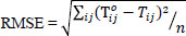
The RMSE is one of the most accurate comparative measures of model performance [65]. RMSE represents the differences between predicted values and observed values with the quadratic mean. It serves to aggregate the magnitudes of the errors in predictions for various data points into a single measure. When the RMSE values are lower correspondence is higher, and 0 would indicate a perfect fit to the data. As the RMSE value gets smaller, it
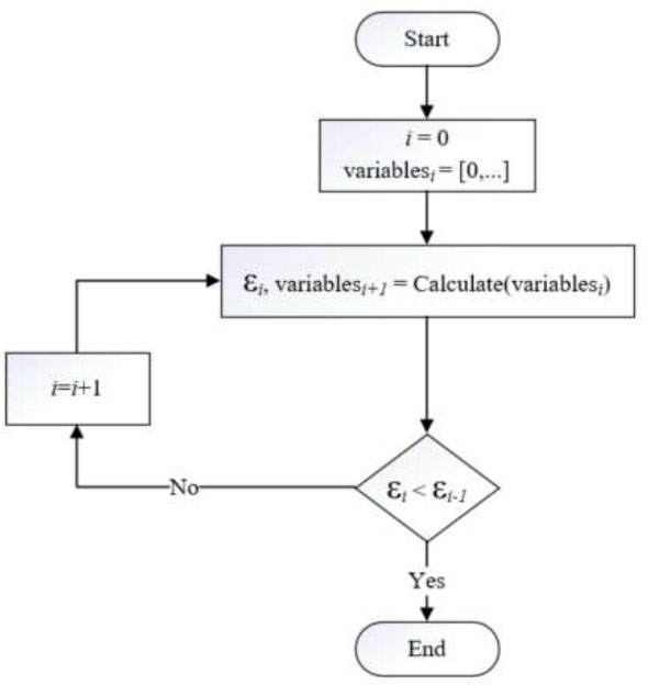
Estimation algorithm.
is determined that the model estimation gets closer to the observed values. The effect of each error on the RMSE is proportional to the squared size of the error; therefore, larger errors have a disproportionately large impact on the RMSE. Accordingly, the RMSE shown in Eq. (18) is sensitive to outliers.
 |
(18) |
In Eq. (18), Tijo represents the number of observed trips, and Tij represents the number of trips obtained as a result of the model. n represents the total number of values compared.
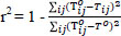
The coefficient of determination (r2) is another widely used measure of model performance. It is a measure of the linear association between observed and predicted values. The r2 value is lies in the range of 0-1. As the value gets closer to 1, the similarity of the model to the observation values increases. It has been determined that in some special cases, the r2 statistic may show insensitivity to error. Therefore, the interpretation of r2 measures should be done with caution [65]. It is presented in Eq. (19).
 |
(19) |
In this equation, Tijo represents the number of observed trips, To represents the average of these observed values, and Tij represents the number of trips obtained as a result of the model.
Mean Travel Cost Error (MTCE) is a macro-level performance measure in trip distribution modelling. It is also employed as a standard calibration procedure for years [66]. In the MTCE, in addition to traffic values, travel costs are also used (Eq. 20). For model and real trips, the trip cost per trip is calculated, and the MTCE is determined by calculating the difference between these values. The calculated value is considered as the deviation value, and the closer the deviation value is to 0, the more realistic the model gives results, regardless of the sign of the deviation.
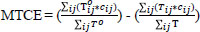 |
(20) |
In Eq. (20), Tijo, To, and Tij represent the same values used in Eq. (19). In addition, is the total number of observed trips, is the total number of estimated trips.
Finally, The Trip Length Distribution (TLD) is determined by calculating the frequency distributions of the travel time or costs for the observed values. It is a macro-level measure for trip distribution modelling, and is used both in the calibration and the model evaluation phases. The TLD obtained by calculating the number of trips within the specified ranges is expected to fit the right-skewed normal distribution in the ideal situation. It is assumed that the TLD graph drawn with the predicted values will remain the same. Trip Length Distribution Root Mean Squared Error (TLD RMSE) measures the root mean squared differences between observed and estimated trip length frequency distributions associated with usual time intervals.
3.3. Empirical Evaluation
In this paper, the model described in Section 3.1 was evaluated with real-world household survey data by using the actual trip information collected for the Eskisehir Master Plan [67]. Eskişehir is a medium-sized city located in the inner parts of Turkey. The network created with TAZs that have sufficient data in the household survey is shown in Fig. (2). As a part of the master plan studies [67] TAZs were determined, and data were collected from more than 30000 households in the 72 TAZs.
In the empirical evaluation, an actual O/D matrix is extracted from the survey and this actual matrix is re-estimated by using both the proposed method and the gravity model. Afterward, for both methods, convergence to the actual values is investigated and the results are compared by using the measures given in Section 3.2. For computational simplicity, this practice is performed by using only a subset of 72 TAZs. The subset contains 5 TAZs selected for different cases. In this empirical analysis, 5 cases are selected: (a) neighboring TAZs, (b) distinct TAZs, (c) TAZs with high travel demand, (d) TAZs with low travel demand, and (e) randomly selected TAZs. Randomly selected TAZs contain arbitrarily selected 5 TAZs while neighboring TAZs include 5 TAZs sharing administrative borders. On the other hand, separate TAZs are defined as TAZs that do not have any administrative borders with each other. The threshold between high and low demand is assumed to be 100 trips/day. Accordingly, for the TAZ group with low demand, the number of trips for every TAZ in the group is less than 100. Parallelly, for the high-demand TAZ group, the number of trips for every TAZ is more than 100.
For all TAZ subsets, a 5x5 O/D matrix was established by using the number of trips obtained from the household surveys. Here, the travel times and costs were determined from the network.
Furthermore, for intra-zonal trips, times and costs are assumed to be zero for computational simplicity. The plots of the cases and TAZs are given in Fig. (3).
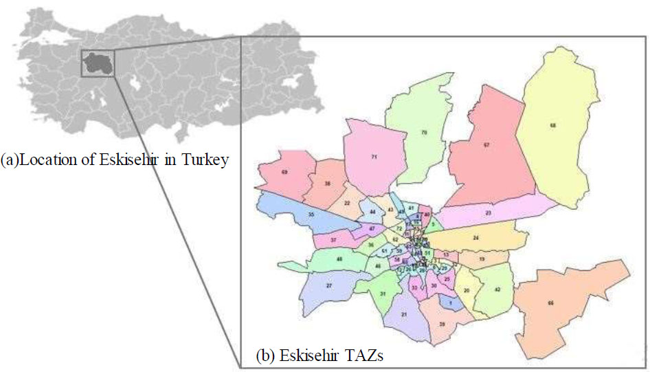
Eskişehir trafic analysis zones (TAZ) [67].
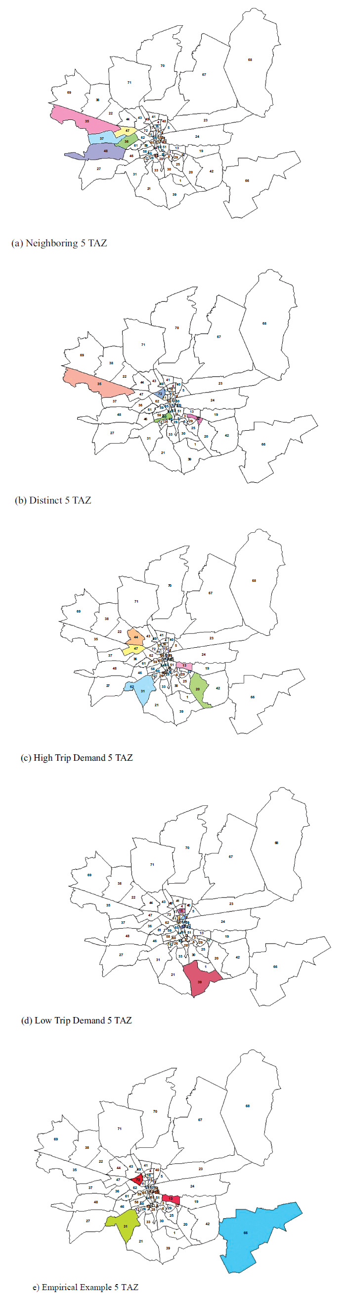
The plot of example cases.
Note: Selected TAZs are colored.
Travel times and travel cost values for the example cases are provided in Table 2. Using these values, empirical examples were calculated employing both the game distribution model and the gravity model. The resulting pairs were then compared using the measures described in Section 3.2.
3.3.1. Calculation with Game Distribution Model and Gravity Method
In the application of the proposed model, which is called the game distribution model, two different types of games were developed as stated in Section 3.1: attraction and production. All best response functions were determined separately with Eqs. (16 and 17). and solved together with the minimization problem defined in Section 3.1.
For each case, all TAZs have their own attraction games, and there are 5 gamers. Similar to attractions, all TAZs have their own production games as well. The final minimization problem contains 25 best response functions for attraction games and 25 best response functions for production games. The determined minimization problem was solved using the algorithm given in Fig. (3). The results provide the total production and total attraction values without the need to apply balancing factors. This is one of the most significant advantages of the proposed model.
The Gravity model, which was introduced in Chapter 2.2, was used as the benchmark model. Trips were calculated with Eq. (11), and the exponential deterrence function that was shown in Eq. (2) was selected for the deterrence function (f(cij)). Many studies have suggested statistical or numerical computational procedures to calibrate the β value in the deterrence function. One of the simplest procedures is to run the model for a wide range of β values, and choose the best β value that optimizes a predetermined goodness-of-fit statistic [68]. In this study, for this purpose, O/D matrices are estimated using all possible β values within the range of 0 and 4. Next, the TLD of every calculation for each β was determined, and every step observed and estimated was compared by using RMSE. The matrix calculated by this β value was determined as the O/D Matrix of the Gravity Model. β optimization was done for all samples, and O/D matrices were calculated with these β values.
Table 2.
| Neighboring 5 TAZ | - | 35 | 36 | 37 | 47 | 48 | |||||
|---|---|---|---|---|---|---|---|---|---|---|---|
| O/D | time | cost | time | cost | time | cost | time | cost | time | cost | |
| 35 | 0 | 0 | 10.55 | 2.66 | 7.83 | 0.69 | 8.44 | 2.16 | 11.38 | 4.07 | |
| 36 | 10.58 | 2.8 | 0 | 0 | 6.74 | 0.83 | 8.27 | 0.91 | 8.31 | 1.6 | |
| 37 | 7.83 | 0.69 | 6.74 | 0.83 | 0 | 0 | 9.56 | 1.07 | 8.56 | 1.61 | |
| 47 | 10.21 | 2.2 | 8.41 | 1.02 | 9.67 | 0.85 | 0 | 0 | 9.24 | 2.44 | |
| 48 | 12.82 | 2.49 | 8.21 | 1.53 | 8.98 | 1.73 | 11.69 | 1.98 | 0 | 0 | |
| Distinct 5 TAZ | - | 11 | 32 | 35 | 60 | 72 | |||||
| O/D | time | cost | time | cost | time | cost | time | cost | time | cost | |
| 11 | 0 | 0 | 11.56 | 1.86 | 12.89 | 3.81 | 9.54 | 1.52 | 5.96 | 0.65 | |
| 32 | 12.24 | 1.99 | 0 | 0 | 18.32 | 6.56 | 7.74 | 1.31 | 13.41 | 3.59 | |
| 35 | 11.21 | 3.75 | 16.64 | 6.09 | 0 | 0 | 14.31 | 5.09 | 9.77 | 3.26 | |
| 60 | 9.65 | 1.57 | 7.96 | 1.74 | 16.69 | 5.37 | 0 | 0 | 10.21 | 1.73 | |
| 72 | 5.96 | 0.65 | 12.38 | 3.63 | 12.41 | 3.44 | 10.5 | 2 | 0 | 0 | |
| High trip demand 5 TAZ | - | 13 | 14 | 31 | 44 | 47 | |||||
| O/D | time | cost | time | cost | time | cost | time | cost | time | cost | |
| 13 | 0 | 0 | 8.83 | 1.5 | 11.72 | 2.54 | 11.77 | 4.16 | 10.92 | 3.91 | |
| 14 | 8.83 | 1.5 | 0 | 0 | 13.52 | 2.83 | 14.95 | 5.26 | 14.1 | 5 | |
| 31 | 11.79 | 2.53 | 13.52 | 2.83 | 0 | 0 | 10.97 | 3.34 | 9.69 | 2.6 | |
| 44 | 12.37 | 4.26 | 15.55 | 5.35 | 9.56 | 3.06 | 0 | 0 | 6.27 | 0.77 | |
| 47 | 11.26 | 3.99 | 14.44 | 5.08 | 9.52 | 2.55 | 6.07 | 0.83 | 0 | 0 | |
| Low trip demand 5 TAZ | - | 10 | 14 | 16 | 39 | 52 | |||||
| O/D | time | cost | time | cost | time | cost | time | cost | time | cost | |
| 10 | 0 | 0 | 4.76 | 0.53 | 5.36 | 0.59 | 15.92 | 3.02 | 6.04 | 0.71 | |
| 14 | 4.76 | 0.53 | 0 | 0 | 7.32 | 0.98 | 16.09 | 3.5 | 6.81 | 0.98 | |
| 16 | 5.36 | 0.59 | 7.27 | 0.96 | 0 | 0 | 17.05 | 5.55 | 7.39 | 1.12 | |
| 39 | 16.23 | 3.57 | 16.44 | 3.71 | 16.7 | 5.49 | 0 | 0 | 14.36 | 3.27 | |
| 52 | 5.87 | 0.7 | 6.08 | 0.79 | 7.33 | 1.11 | 13.87 | 2.7 | 0 | 0 | |
| Randomly selected TAZ TAZs | - | 13 | 31 | 45 | 66 | 72 | |||||
| O/D | time | cost | time | cost | time | cost | time | cost | time | cost | |
| 13 | 0 | 0 | 11.72 | 2.54 | 5.65 | 0.80 | 11.77 | 4.02 | 11.41 | 3.22 | |
| 31 | 11.79 | 2.53 | 0 | 0 | 11.47 | 2.48 | 17.65 | 8.28 | 8.86 | 2.78 | |
| 45 | 5.65 | 0.80 | 11.35 | 2.48 | 0 | 0 | 13.83 | 4.51 | 9.79 | 1.45 | |
| 66 | 12.06 | 4.09 | 17.88 | 8.31 | 13.97 | 4.39 | 0 | 0 | 15.40 | 5.82 | |
| 72 | 10.22 | 3.66 | 10.16 | 2.96 | 9.9 | 1.41 | 14.29 | 6.29 | 0 | 0 | |
| O/D | 35 | 36 | 37 | 47 | 48 | |||||
|---|---|---|---|---|---|---|---|---|---|---|
| - | Observed | GDM Gravity |
Observed | GDM Gravity |
Observed | GDM Gravity |
Observed | GDM Gravity |
Observed | GDM Gravity |
| 35 | 250 | 272 211 |
1 | 0 20 |
22 | 15 33 |
74 | 62 75 |
2 | 0 9 |
| 36 | 2 | 2 4 |
39 | 35 29 |
7 | 11 7 |
8 | 0 14 |
1 | 9 3 |
| 37 | 51 | 46 79 |
88 | 83 77 |
312 | 306 283 |
107 | 139 107 |
16 | 0 29 |
| 47 | 18 | 7 17 |
5 | 18 19 |
11 | 0 14 |
268 | 280 246 |
2 | 0 9 |
| 48 | 6 | 0 16 |
42 | 39 31 |
10 | 30 26 |
24 | 0 38 |
116 | 129 87 |
The Game Distribution Model (GMD) and gravity model O/D matrices for all example cases are given in the tables below. Table 3 contains the calculated O/D matrix for neighboring TAZs. Similarly, Tables 4, 5, 6, and 7 include the model results for discrete, high trip demand, low trip demand, and randomly selected cases, respectively.
4. RESULTS
The Game Distribution Model (GMD) and the Gravity Model were solved for each case, and then each model’s results were compared with goodness-of-fit statistics described in Chapter 3.2. The results are shown in Tables 8 and 9.
According to the comparison of micro-level goodness-of-fit statistics given in Table 5, r2 values for both models are over 0.80, and the results are statistically sufficient. When analyzing the results from the perspective of RMSE, the Game Distribution Model outperforms the Gravity Model in two specific cases, while overall, the results for both models are relatively very close.
| O/D | 11 | 32 | 35 | 60 | 72 | |||||
|---|---|---|---|---|---|---|---|---|---|---|
| - | Observed | GDM Gravity |
Observed | GDM Gravity |
Observed | GDM Gravity |
Observed | GDM Gravity |
Observed | GDM Gravity |
| 11 | 56 | 57 55 |
4 | 6 6 |
6 | 10 9 |
3 | 9 9 |
33 | 19 24 |
| 32 | 0 | 4 5 |
79 | 62 61 |
1 | 0 3 |
4 | 21 13 |
4 | 0 6 |
| 35 | 15 | 0 12 |
3 | 0 4 |
250 | 230 235 |
7 | 0 7 |
4 | 49 22 |
| 60 | 16 | 20 20 |
12 | 44 29 |
18 | 0 10 |
171 | 137 142 |
7 | 24 25 |
| 72 | 51 | 57 47 |
4 | 0 14 |
12 | 47 28 |
5 | 22 20 |
251 | 206 222 |
| O/D | 13 | 14 | 31 | 44 | 47 | |||||
|---|---|---|---|---|---|---|---|---|---|---|
| - | Observed | GDM Gravity |
Observed | GDM Gravity |
Observed | GDM Gravity |
Observed | GDM Gravity |
Observed | GDM Gravity |
| 13 | 317 | 252 284 |
15 | 106 41 |
42 | 18 34 |
26 | 20 26 |
22 | 26 36 |
| 14 | 72 | 171 95 |
529 | 460 471 |
31 | 46 46 |
13 | 0 27 |
32 | 0 38 |
| 31 | 54 | 42 50 |
8 | 0 30 |
714 | 618 651 |
58 | 84 57 |
40 | 130 86 |
| 44 | 25 | 0 41 |
9 | 0 18 |
58 | 137 89 |
492 | 438 474 |
194 | 203 156 |
| 47 | 23 | 26 22 |
5 | 0 10 |
16 | 42 39 |
59 | 106 61 |
268 | 198 239 |
| O/D | 10 | 14 | 16 | 39 | 52 | |||||
|---|---|---|---|---|---|---|---|---|---|---|
| - | Observed | GDM Gravity |
Observed | GDM Gravity |
Observed | GDM Gravity |
Observed | GDM Gravity |
Observed | GDM Gravity |
| 10 | 44 | 28 43 |
0 | 8 3 |
4 | 16 2 |
0 | 0 0 |
12 | 9 11 |
| 14 | 1 | 3 1 |
16 | 7 14 |
0 | 2 0 |
0 | 0 0 |
0 | 3 2 |
| 16 | 0 | 11 1 |
2 | 5 0 |
38 | 22 39 |
1 | 0 0 |
3 | 6 3 |
| 39 | 0 | 0 0 |
0 | 0 0 |
0 | 0 0 |
43 | 44 44 |
1 | 0 0 |
| 52 | 0 | 0 0 |
0 | 0 0 |
0 | 0 0 |
0 | 0 0 |
2 | 1 2 |
In this study, two macro-level goodness-of-fit statistics are calculated, and the results are shown in Table 6. The Game Distribution Model has better results in almost all cases according to the MTCE measure. For the TLD-based comparison at the macro level, the TLD graphics of all predictions with both models were prepared. Next, TLD RMSE values were calculated by referring to the actual and predicted TLDs. When the last two columns in Table 6 are considered, in 2 of 5 cases, the proposed model provided better results. This should be considered a success for The Game Distribution Model, while the basis of calibration in the Gravity Model is TLD. In Fig. (4), the TLD graphics for all example cases are plotted. All graphics (Fig. 4a-e) show that both models give results close to the observed values. In the game distribution model, unlike gravity theory, TLD values are not used directly. Despite this, the closeness of the results can be considered a success for the proposed model.
5. DISCUSSION
The general purpose of this study was to estimate the OD matrices with the Game Theory and contribute to the literature by representing its potential use in the Trip Distribution Modelling. After thorough investigations, the present study demonstrates the applicability of the proposed model, with its outputs yielding better or comparable goodness-of-fit statistics compared to the classic Gravity Model. This indicates that the Game Distribution Model can serve as a replacement for the Gravity Model in the Trip Distribution step of the Four-Step Travel Demand Model.
| O/D | 13 | 31 | 45 | 66 | 72 | |||||
|---|---|---|---|---|---|---|---|---|---|---|
| - | Observed | GDM Gravity |
Observed | GDM Gravity |
Observed | GDM Gravity |
Observed | GDM Gravity |
Observed | GDM Gravity |
| 13 | 317 | 332 385 |
42 | 41 1 |
4 | 2 1 |
16 | 6 1 |
9 | 7 0 |
| 31 | 54 | 47 0 |
714 | 764 811 |
1 | 0 0 |
11 | 0 0 |
31 | 0 0 |
| 45 | 3 | 4 7 |
6 | 0 1 |
17 | 20 19 |
0 | 0 0 |
1 | 3 0 |
| 66 | 10 | 0 0 |
14 | 0 0 |
0 | 0 0 |
144 | 169 169 |
1 | 0 0 |
| 72 | 25 | 26 17 |
87 | 58 52 |
0 | 0 2 |
4 | 0 4 |
251 | 283 293 |
| - | r2 | RMSE | ||
|---|---|---|---|---|
| Game Distribution Model | Gravity Model |
Game Distribution Model | Gravity Model | |
| Neighboring | 0.98 | 0.98 | 12.57 | 15.85 |
| Distinet | 0.94 | 0.98 | 20.00 | 12.48 |
| High trip demand | 0.94 | 0.99 | 51.13 | 26.34 |
| Low trip demand | 0.80 | 0.99 | 6.21 | 1.06 |
| Random selected | 0.99 | 0.98 | 16.56 | 31.03 |
| - | MTCE | TLD RMSE | ||
|---|---|---|---|---|
| Game Distribution Model | Gravity Model |
Game Distribution Model | Gravity Model | |
| Neighboring | 3.54 | -9.12 | 0.02 | 0.04 |
| Distinet | -6.91 | -8.77 | 0.06 | 0.05 |
| High trip demand | -19.39 | -27.54 | 0.06 | 0.03 |
| Low trip demand | -0.92 | 0.30 | 0.13 | 0.01 |
| Random Selected | 21.17 | 33.00 | 0.03 | 0.06 |
The main advantages of the Game Distribution Model are as follows:
- The proposed model directly uses data from household surveys or networks such as production attraction values, travel costs, etc. However, the Gravity Model needs different parameters, like the generalized travel cost function.
- The proposed model does not use any correction coefficients (socio-economic adjustment factors- K) that account for the difference between actual results and predictions used in the Gravity Model.
- The proposed Model has flexibility in defining the trip utility. The best response functions can accommodate a variety of variables such as employment for home base work trips or shopping mall area in destination TAZ for non-home base trips etc.
- The model also has flexibility about the cost function; travel time, travel cost, or any deterrence parameter can be used in the proposed model.
The most important advantage of The Game Distribution Model is that the model uses the most basic Game Theory approach (static and complete information) but can be improved by incorporating the concept of incomplete information in future studies. This will provide a more realistic approach instead of assuming that the passengers have accurate information about all TAZs, similar to classic distribution models.
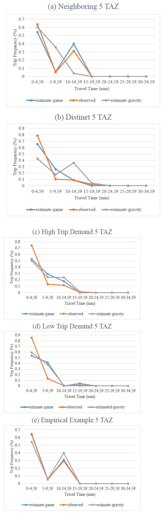
TLD comparison for example cases.
CONCLUSION
Besides these advantages, the complexity of the application can be mentioned as the main disadvantage of the Game Distribution Model. The Gravity Model is still simple and efficient. Considering advancements in programming, this disadvantage can be addressed by solving the minimization problem using suitable software solutions.
Further research can explore designing some new features with additional utility or cost variables, such as zonal land use variables or a geographical barrier. The model can be examined in examples with different numbers of TAZs and can be recommended for certain scales. It can be investigated to find out which model might be used for different sized zones.
AUTHORS’ CONTRIBUTION
It is hereby acknowledged that all authors have accepted responsibility for the manuscript's content and consented to its submission. They have meticulously reviewed all results and unanimously approved the final version of the manuscript.
LIST OF ABBREVIATIONS
| TAZ | = Traffic Analysis Zone |
| GRG | = Generalized Reduced Gradient |
| RMSE | = Root Mean Squared Error |
| Coefficient of Determination r2 | = 2 is a upper index |
| MTCE | = Mean Travel Cost Error |
| TLD | = Trip Length Distribution |
| O/D | = Orijin/Destination |
| GDM | = Game Distribution Model |
AVAILABILITY OF DATA AND MATERIALS
The data and supportive information are available within the article.
ACKNOWLEDGEMENTS
The authors thank the kind help of Esma Morgül and Mustafa Gündoğar.

