All published articles of this journal are available on ScienceDirect.

Integrating Ensemble Machine Learning and Structural Equation Modeling to Predict and Explain Biking Demand in Kigali: A Data-driven Approach for Sustainable Urban Mobility
Authors Info & Affiliations
Abstract
Introduction
Biking-both shared and non-shared-has become a vital component of sustainable urban mobility across African cities like Kigali. Despite this progress, empirical research and demand modeling of biking behavior remain limited. This study predicts and explains biking behavior in Kigali by integrating advanced ensemble machine learning (ML) techniques with structural equation modeling (SEM).
Methods
A dataset of 6,386 observations was compiled by merging survey responses on biking with secondary data on weather and air quality. Both traditional statistical and advanced ensemble models were developed for comparison. The dataset was partitioned into training (70%) and testing (30%) subsets, with correlation-based and model-based feature selection applied. SEM examined latent constructs representing spatial, social-demographics, temporal, environmental, and attitudinal factors.
Results
Ensemble ML models substantially outperformed traditional approaches, with random forest and XGB classifiers achieving the highest predictive performance. The SEM demonstrated good model fit and explained the variance in biking frequency. Perceived station accessibility emerged as the strongest determinant of biking behavior, while temporal and environmental factors indirectly influenced demand patterns.
Discussion
The combination of ML and SEM has revealed a coexistence of accurate prediction and behavioral insight. Accessibility emerged as central to biking uptake, highlighting the potential of station placement and spatial equity. Indirect effects of temporal and environmental conditions highlight the impact of user perceptions in shaping biking demand.
Conclusion
Integrating ensemble ML and SEM provides predictive robustness and behavioral insight. The findings highlight that improving spatial accessibility and adopting adaptive urban planning strategies enhance sustainable biking uptake.
1. INTRODUCTION
The transportation sector is undergoing a transformation toward sustainable and inclusive mobility aligned with the SDGs (United Nations Sustainable Development Goals) and the New Urban Agenda [1]. Among the low-emission alternatives to motorized transport, biking-both shared and non-shared-has emerged as a viable and equitable mode for urban mobility. While bike sharing systems were formally introduced in the Netherlands in 1965 [2], their adoption has accelerated globally and is now gaining momentum in research focused on emerging African cities, such as Kigali, Rwanda [3], Kumasi in Ghana [4], and Quelimane in Mozambique [5].
Despite this, the modeling of biking demand in African cities remains underdeveloped, limiting the ability of policymakers to implement data-driven planning for non-motorized transport infrastructure. Traditional statistical approaches-such as Bayesian Conditional Autoregressive [6], k-nearest neighbors (KNN) and support vector machines (SVM) [7], and multinomial logit models [8] have frequently been used to model bike sharing demand. However, these models often underperform when dealing with nonlinear relationships, high-dimensional feature spaces [9, 10], and multicollinearity [11], which are common in transport datasets. Additionally, ensemble models, such as Random Forest [12], stacking classifiers [13], Extreme Gradient Boosting (XGBoost) [14], and Light Gradient Boosting Machine (LightGBM) [15] combine multiple learners to improve accuracy beyond what a single model can achieve. The above models have achieved a superior performance in demand prediction involving complexes along with high-dimensional data. However, ensemble models typically lack the ability to analyze causal or structural relationships among factors influencing bike sharing demand, which limits their explanatory power compared to theory-driven models like SEM (Structural Equation Modeling) [16].
To bridge the gap, this study is the first research in transportation integrating advanced ensemble machine learning models, including XGBoost, Random Forest, and a Stacking Classifier-with Structural Equation Modeling (SEM) to predict and explain biking demand, which existing research has failed to achieve. This dual-method framework provides both high predictive performance and behavioral interpretability, which machine learning or SEM cannot do alone. The analysis is based on a dataset of 6,386 observations, merging primary survey data on biking demand with secondary weather and air quality variables. This dataset enables robust predictive modeling in a data-scarce context and captures both objective and perceptual drivers of biking behavior.
The findings reveal that ensemble machine learning models significantly outperform traditional approaches, achieving predictive accuracies between 97% and 99%, compared to 42%–82% for conventional models. The SEM results yielded strong model fit indices (RMSEA = 0.036, CFI = 0.932) and explained 77.1% of the variance in biking frequency. Notably, spatial accessibility emerged as the most influential latent factor (β = 0.878, p < 0.001), with perceived station access having the strongest effect (β = 0.995). While environmental and temporal variables played a critical role in the predictive models, their direct causal pathways in the SEM were more limited. These results contribute actionable evidence to support low-carbon urban transport systems by guiding policy interventions, such as investment in car-free corridors, station accessibility, and seasonally adaptive cycling infrastructure.
The methodological framework used in this research is designed for replicability and scalability across other rapidly urbanizing African cities-such as Nairobi in Kenya, Kampala in Uganda, and Dar es Salaam in the United Republic of Tanzania, where similar data constraints and urban challenges exist. This paper begins by describing the materials and methods, followed by a presentation of the results. It then discusses the key findings and concludes with policy implications.
2. MATERIALS AND METHODS
2.1. Study Area
Rwanda is an East African country with Tanzania to the East, Burundi to the South, Uganda to the North, and the DRC (Democratic Republic of the Congo) to its West. In recent decades, Rwanda has experienced substantial demographic growth and urban expansion. Its population has been growing at an annual rate of approximately 2.86%, while the urbanization rate increased from 18.4% in 2012 to an estimated 35% by 2024 [17].
Kigali, the case study, is the capital of Rwanda with a population corresponding to 1,745,555 on 730 square kilometers and projected to reach 3.8 million by 2035 [18]. Compared to other East African cities, Kigali has a moderate population density, making it more suitable for planning non-motorized transport (NMT) easily. Its demographic characteristics and hilly topography also present promising opportunities for research and implementation of cycling initiatives.
Kigali has developed an NMT master plan to serve as its guiding framework. To date, the city has constructed 215 kilometers of dedicated cycling lanes, with plans to expand the network to 418 kilometers by 2050 [19]. These lanes are physically separated from motor vehicles and pedestrian pathways to enhance safety and encourage cycling. In addition, the city has introduced regular car-free days and established car-free zones, such as the Imbuga City Walk, to reduce greenhouse gas emissions [20]. Moreover, the city launched the first public bike sharing program in 2021 and has encouraged its employees to reduce reliance on motorized transport by providing electric bicycles, free of charge and maintenance [21].
2.2. Sample Strategies
Table 1 summarizes how data were collected from three districts of the city, and the sample size for each district was proportional to its population. A total sample of 6,386.00 was determined, then distributed to those three districts as per Table 1.
| Districts of the City | % of Population in Each District | Sample Size for Each District |
|---|---|---|
| Gasabo | 50.39% | 3,218 |
| Kicukiro | 28.17% | 1,799 |
| Nyarugenge | 21.44% | 1,369 |
Table 2 identifies temporal, environmental, geographic, demographic, and behavioral factors influencing biking demand in Kigali. Bike users were categorized as non-shared, bike-sharing, or both. Rainfall, humidity, and poor air quality (high PM2.5, NO2, O3) reduced biking activity. Nyarugenge had the highest bike-sharing uptake due to better connectivity and station density, while Gasabo and Kicukiro favored non-shared bikes.
2.3. Weather Data and Air Quality Data
Daily weather and air quality data were collected between 14th December 2022 and 29th February 2024, aligned with the period of survey data collection. Weather data were collected from Meteo Rwanda in Kigali city stations, which included solar radiation intensity, humidity, rainfall, temperature variations, and wind speed. These variables were selected due to their effects on the comfort and safety of the riders [21]. Air quality data were collected from REMA (Rwanda Environment Management Authority) at its Kigali stations, including CO (carbon monoxide), PM2.5 (particulate matter), NO2 (nitrogen dioxide), and CO2 (carbon dioxide). These data were selected to understand how they affect bike-sharing adoption [22].
2.4. Data Pre-processing
Initially, all variables were converted to their appropriate data types. Irrelevant columns were identified through univariate analysis and subsequently removed. To maintain data integrity, missing values and outliers were carefully addressed. Records with more than 10% missing data were excluded, while missing values in numerical variables were estimated using time-based linear interpolation, leveraging the date-time index to fill gaps based on temporal progression [23].
| Variable | Name | Description | |
|---|---|---|---|
| Dependent Variable | Biking Preference | - Non-shared bike | |
| - Bike sharing | |||
| - Both shared and non-shared | |||
| Independent Variables | Category | Variable Name | Description / Categories |
| - | Temporal | Day | Days of the week |
| - | - | Month | Months of the year |
| - | - | Year | 2022 to 2024 |
| - | Weather & Air Quality | Relative Humidity | Solar radiation (W/m2) |
| - | - | Wind Speed | % |
| - | - | Radiation | m/s |
| - | - | Wind Direction | Degrees (°N) |
| - | - | Cloud Opacity | % |
| - | - | Max Temperature | °C |
| - | - | Min Temperature | °C |
| - | - | Rainfall | mm |
| - | - | Atmospheric Pressure | hPa |
| - | - | SO2, CO, NO2, O3, PM10, PM2.5 | Air pollutants (μg/m3 or ppb) |
| - | Geographic | District | Gasabo, Kicukiro, Nyarugenge |
| - | Demographic | Age | Below 18, 19–24, 25–30, 31–36, Above 44 |
| - | - | Gender | Male, Female, Other |
| - | - | Household Income | Low, Lower-middle, Upper-middle, High |
| - | - | Education Level | Primary, Secondary, Tertiary |
| - | - | Occupation | Student, Employed, Unemployed, Retired |
| - | Behavioral / Preferences | Average Bike Trip Duration | <30 min, 30–45 min, 45–60 min |
| - | - | Satisfaction Level with Biking Services | Very satisfied, Satisfied, Neutral, Dissatisfied |
| - | - | Distance to Nearest Bike Sharing Station | <500m, 1–3 km, >3 km |
| - | - | Influencing Factors | Infrastructure, Convenience, Cost-effectiveness, Safety, Accessibility, Environmental Concerns |
| - | - | Desired Biking Features | Protected lanes, Signals, Bike racks, and Station availability |
| - | - | Infrastructure Quality & Accessibility | Excellent, Good, Fair, Poor, Very Poor |
2.5. Exploratory Data Analysis
Exploratory data analysis (EDA) was conducted to examine the characteristics, distributions, and patterns within the dataset. Univariate analysis using histograms was applied to visualize the distributions of numerical and categorical variables, revealing, for instance, skewed distributions in temperature and PM10 levels [24]. Bivariate analysis was performed to identify relationships between key variable pairs, highlighting strong correlations between NO2 and CO concentrations [25]. Temporal analysis was employed to explore trends in weather and air quality variables over the study period, showing seasonal variations in temperature, humidity, and pollutant concentrations. Python with scikit-learn was used for data processing and analysis, while AMOS facilitated structural equation modeling.
2.6. Selection of Features
Feature selection was conducted in two stages. First, multicollinearity was assessed using Pearson correlation plots, and for highly correlated pairs (correlation > 0.7), only one feature was retained [26, 27]. Second, iterative model-based procedures were applied to evaluate feature importance, with ensemble models used to identify variables that could mask the contribution of others [28, 29]. Based on these analyses, less informative or over-generalized features-including 'bike sharing influencing factors', 'year', 'biking features', 'PM10', 'wind speed', 'cloud opacity', 'wind direction', 'solar radiation', 'atmospheric pressure', 'gender', 'minimum temperature', 'relative humidity', 'household income', 'education level', 'NO2', and 'SO2'-were excluded from model training.
2.7. Correlation Test
This test was used to assess the correlation between variables, with a strength ranging from 1 to -1: 1 indicates a positive correlation, 0 indicates no correlation, and -1 indicates a negative correlation.
2.8. Modelling
• Logistic Regression: This model is known for classification problems, where it models the probability that a given variable belongs to a particular class with values between 0 and 1 of the response variables [30]. This research used a multi-class classification approach in which a binary classifier is trained for each class against all other classes separately; the predicted probabilities were obtained during the multi-class logistic regression model training phase [31].
• Support Vector Machine (SVM): This model is famous for classification analysis. The SVM was chosen for its effectiveness with high-dimensional data [32].
• Random Forest Model: A random subset of the training data is constructed using each tree and a random subset of all features. In this research, with replacements from the original dataset, a random forest was implemented by taking random samples to create a bootstrapped dataset of the same size. Subsequently, at each split in a decision tree, a subset of features was randomly selected from the complete set of features [33].
• Stacking Classifier: Stacking is an ensemble learning technique that combines multiple machine learning models to obtain predictions that are used as input features for a meta-classifier [33]. This research used a stacking classifier to fit several baseline models, including KNN, Naïve Bayes, SVM, and Logistic Regression [34, 35]. Then, the predictions of those classifiers were used to train and generate predictions.
• Structural Equation Modeling (SEM):It is a powerful statistical approach used to explore complex relationships among observed and latent variables. By combining aspects of factor analysis and multiple regression within a single framework, SEM allows researchers to test theoretical models that incorporate both measurement and structural components. SEM is particularly prevalent in disciplines such as education and the social sciences because it can model latent constructs and evaluate hypothesized causal pathways [36-38].
Structural Equation Modeling (SEM) was used to evaluate the fit of the proposed model to the observed data [39]. Model fit was assessed using the Comparative Fit Index (CFI), Tucker–Lewis Index (TLI), and Root Mean Square Error of Approximation (RMSEA), with commonly accepted thresholds of CFI/TLI ≥ 0.95 and RMSEA ≤ 0.06 [40-42].
2.9. Model Metrics
The ensemble machine learning models were evaluated through cross-validation, employing the accuracy metric to gauge their predictive performance. The outcome of each fold's accuracy scores was stored, and the mean and standard deviation were printed on the model's effectiveness [43]. In parallel, the structural equation model (SEM) was evaluated using multiple model fit indices, such as the Root Mean Square Error, Comparative Fit Index, Tucker-Lewis Index, Chi-square statistics, and Normed Fit Index. These SEM metrics complemented the machine learning evaluations by validating the structural relationships between latent constructs. Together, the combination of predictive metrics from ensemble learning and explanatory metrics offered a robust framework for understanding and predicting biking demand [40]. Figure 1 shows how each method was used.
3. RESULTS
3.1. Descriptive Statistics
Based on a total of 6,386 observations, the recorded maximum temperature ranged from 25.8°C to 61.2°C, with a mean of 38.4°C, reflecting both the central tendency and variability of this key environmental variable. Rainfall levels were relatively low, with an average of 2.6 mm and a maximum of 21.2 mm, indicating limited precipitation in the study area. In terms of air quality, the average ozone concentration was 20.8, while PM2.5 levels averaged 42.8, peaking at 127.2, signaling considerable air pollution across the study period.
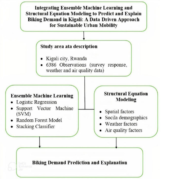
Conceptual framework.
| Traditional Statistical Models | Ensemble Models | ||||
|---|---|---|---|---|---|
| Logistic regression | SVM | Random forest | XGB | Stacking classifier | |
| Accuracy | 42% | 82% | 98% | 99% | 94% |
| Macro avg (precision) | 42% | 68% | 99% | 99% | 87% |
| Weighted avg(precision) | 71% | 88% | 98% | 99% | 94% |
3.2. Modelling Results
The findings in Table 3 demonstrate that ensemble machine learning models-Random Forest, XGBoost, and Stacking-significantly outperform traditional methods in predicting biking demand. While logistic regression achieved only 42% accuracy and SVM 82%, ensemble models reached up to 99% accuracy and high precision, effectively capturing complex, nonlinear biking behavior. Their reliability makes them valuable for optimizing bike-sharing systems, guiding infrastructure planning, and supporting policies that promote active transport.
3.3. Features Associated with Demand
The Random Forest model results shown in Fig. (2) indicate that environmental factors, marital status, age, monthly income, and household number are the most critical factors in predicting biking demand in Kigali. These insights help urban planners and mobility service providers to prioritize air quality management, weather-adaptive strategies, and seasonal planning to better align bike sharing operations with user demand.
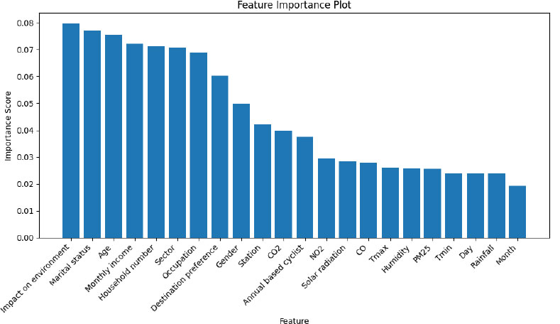
Feature importance.
The model fit indices (Table 4) indicate that the structural equation model for biking demand is statistically robust. Despite a significant χ2 value due to the large sample size (n = 6,386), other indices demonstrate good fit: RMSEA = 0.036, CFI = 0.932, and TLI = 0.910. These results suggest that the model adequately captures the relationships between observed and latent variables influencing biking demand.
The results in Table 5 present the standardized regression weights for the main factors influencing ride frequency, offering key insights into what drives biking demand.
• The most significant predictor is spatial factors (β = 0.878, p < 0.001), which show a strong and statistically significant positive relationship with ride frequency. This suggests that proximity to bike sharing stations, road connectivity, and availability of biking infrastructure have a substantial impact on how frequently people use bikes.
• On the other hand, sociodemographic variables, such as household income (β = -0.001, p = 0.879), age, and occupation, as well as environmental factors (β = 0.002, p = 1.000), and time-of-day ride preferences (β = -0.006, p = 0.347) do not show a significant influence on ride frequency.
Table 6 shows the extent to which the model explains variance in key variables, indicating its predictive strength. Ride frequency has a high explained variance (R2 = 0.771), demonstrating strong predictive capacity, particularly due to spatial-related factors. Accessibility and rainfall show exceptionally high explained variance (R2 = 0.990), highlighting their significant influence on biking behavior. Other variables, such as education level and age, exhibit moderate explained variance, suggesting a lesser but still relevant impact.
Table 7 shows how latent socio-demographic factors relate to observed indicators like age, education, and employment in explaining biking demand. Age and education are most influential, but overall socio-demographics have a limited effect on ride frequency. Individuals with primary education bike mostly for work, while those with secondary education exhibit diverse purposes, including employment, studies, unemployment, and retirement.
In Fig. (3), the model demonstrates that biking frequency is not determined by a single factor but by a network of interrelated influences, which machine learning cannot provide in feature importance. The integration of latent variables helps capture underlying constructs that are not directly measurable but significantly shape cycling behavior.
| Fit Index | Value | Recommended Threshold | Interpretation |
|---|---|---|---|
| Chi-square (χ2) | 784.440 | Low (non-significant ideal) | Acceptable with large sample |
| Degrees of Freedom (df) | 69 | - | - |
| χ2/df | 11.369 | < 5 (ideal), < 3 (good) | High, but tolerable |
| RMSEA | 0.036 | < 0.08 (acceptable), < 0.05 (good) | Good fit |
| CFI | 0.932 | ≥ 0.90 | Acceptable fit |
| TLI | 0.910 | ≥ 0.90 | Acceptable fit |
| NFI | 0.926 | ≥ 0.90 | Acceptable fit |
| PCFI | 0.706 | > 0.50 | Parsimonious model |
| Hoelter (.05) | 893 | > 200 | Strong sample size adequacy |
| Path | Standardized Estimate (β) | Significance (P) |
|---|---|---|
| Ride Frequency ← Spatial Factors | 0.878 | *** |
| Ride Frequency ← SOCIODEMOGRAPHICS | -0.005 | 0.526 |
| Ride Frequency ← Environmental Factors | 0.002 | 1.000 |
| Ride Frequency ← Time of Day Ride Pref | -0.006 | 0.347 |
| Ride Frequency ← Gender | -0.013 | 0.045 |
| Ride Frequency ← Household Income | -0.001 | 0.879 |
| Variable | R2 (Explained Variance) |
|---|---|
| Ride Frequency | 0.771 (77.1%) |
| Education Level | 0.425 |
| Age of respondents | 0.372 |
| Employment Status | 0.006 |
| ZAccess Perception | 0.990 |
| Z_Rainfall Gitega | 0.990 |
| Other variables | 0.000 |
| Latent Variable | Observed Indicators | Notes |
|---|---|---|
| Socio-demographics | Education Level, Age, Employment Status | Strong Age & Education loadings |
| Spatial Factors | Distance to Station, Infrastructure Quality, Access Perception | Access Perception is very strong (β = .995) |
| Environmental Factors | Rainfall, Temperature, Sunny Weather | Rainfall strong (β = .995), others weak |
The high performance in ensemble machine learning models in Table 8 is broadly consistent with the results reported in previous research. Random Forest model in this research achieved 98% accuracy and a 99.8% AUC, outperforming the accuracies reported in previous studies [44, 45]. In terms of AUC, the Random Forest model in this research outperformed another research [46]. This Support Vector Machine (SVM) model recorded 82% accuracy and 84% AUC, lower compared to a previous study [47]. In terms of AUC, this stacking model outperformed the 90.4% benchmark reported by a recent study [48]. This stacking classifier attained 94% accuracy and a 98% AUC, which compares favorably with the 94.4% and 97% accuracies reported recently [49, 50], respectively. Despite achieving high accuracy in other studies [51, 52], the study successfully incorporated features but failed to report the relationships among constructs, which highlights a limitation of the machine learning approach.
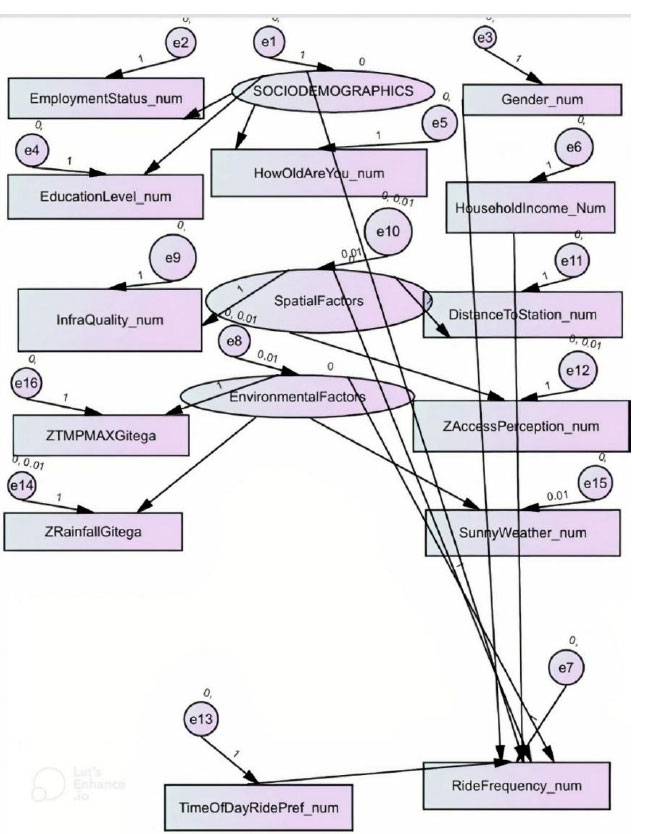
SEM path diagram for observed variables, latent variables, and error terms.
4. DISCUSSION
• The findings indicated that ensemble machine learning models outperformed traditional statistical models in predicting bike-sharing demand. Logistic Regression achieved 42% accuracy and Support Vector Machine 82%, whereas XGBoost, Random Forest, and Stacking Classifier reached 99%, 98%, and 94%, respectively. This demonstrates the superior ability of ensemble models to capture nonlinear and interactive relationships among variables, along with automatic feature importance ranking, which traditional models cannot achieve.
• Despite their predictive strength, ensemble models failed to reveal causal pathways and latent behavioral constructs, whereas Structural Equation Modeling (SEM) effectively captured them. Feature importance analysis highlighted spatial and environmental factors-particularly distance to bike stations, infrastructure quality, and perceived accessibility-as key determinants of biking demand. High loadings on perceived access and rainfall suggest that accessibility perception and adverse weather conditions strongly influence biking frequency.
• SEM results (RMSEA = 0.036, CFI = 0.932, TLI = 0.910) reinforced the robustness of these relationships, revealing spatial factors (β = 0.878, p < 0.001) as the only significant predictors of ride frequency. This contrasts with prior studies emphasizing sociodemographic influences such as age, gender, and income. The high explanatory power (R2 = 0.771) further indicates that accessibility-related variables, rather than user characteristics, predominantly drive bike-sharing participation in Kigali.
• By combining ensemble machine learning (ML) models with Structural Equation Modeling (SEM), ensemble models captured complex, non-linear relationships and key predictors, while SEM clarified behavioral pathways and causal mechanisms. These findings corroborate prior studies showing that ensemble ML outperforms traditional statistical approaches [53, 54]. Unlike previous research, this study identified accessibility and weather as dominant determinants in Kigali, offering a novel, context-specific framework that unites predictive accuracy with interpretive depth-valuable for sustainable urban mobility planning and policy. While these results provide actionable insights, the study is limited by its focus on Kigali and by its reliance on cross-sectional survey data, which may not capture seasonal or long-term behavioral changes.
• Additionally, this research has demonstrated how the integration of AI, behavioral modeling, and SDG-aligned urban planning provides both predictive power and policy insight for advancing sustainable mobility-a practical manifestation of the interdisciplinary sustainability goals explored across the following four studies [55-58].
CONCLUSION
This study demonstrated that ensemble machine learning models, particularly Random Forest and Stacking Classifier, outperform traditional statistical models in predicting bike-sharing demand in Kigali, achieving up to 98% and 99.8% accuracy. These models effectively capture complex, non-linear relationships among biking behavior, spatial factors, and environmental conditions, which traditional models are unable to capture. However, ensemble models alone cannot reveal causal pathways or latent behavioral constructs, which Structural Equation Modeling (SEM) successfully elucidated. SEM results identified spatial accessibility, perceived access, and rainfall as dominant determinants of biking frequency, emphasizing the importance of infrastructure quality and weather sensitivity. By integrating ensemble prediction with SEM-based causal interpretation, this research provides both predictive accuracy and explanatory depth. These findings advance sustainable urban transportation and offer a robust methodological framework linking data-driven demand forecasting with behavioral understanding, guiding evidence-based interventions, such as weather-adaptive operations, infrastructure expansion, and accessibility-focused planning. This approach not only informs local policy in Kigali but also establishes a transferable model for other urban contexts, advancing theory and practice in sustainable mobility.
AUTHORS’ CONTRIBUTIONS
The authors confirm contribution to the paper as follows: J.M.V.N.: Written the paper under the supervision of Hannibal Bwire and Alphonse Nkurunziza.
LIST OF ABBREVIATIONS
| CFI | = Comparative Fit Index |
| CO | = Carbon Monoxide |
| CO2 | = Carbon Dioxide |
| DRC | = Democratic Republic of the Congo |
| EDA | = Exploratory data analysis |
| KNN | = K-nearest Neighbors |
| ML | = Machine Learning |
| NMT | = Non-Motorized Transport |
| NO2 | = Nitrogen Dioxide |
| O3 | = Ozone |
| PM10 | = Particulate Matter with particles measuring 10 micrometers |
| PM2.5 | = Particulate matter with particles measuring 2.5 micrometers |
| RMSEA | = Root Mean Square Error of Approximation |
| SDGs | = United Nations Sustainable Development Goals |
| SEM | = Structural Equation Modeling |
| SO2 | = Sulfur Dioxide |
| SVM | = Support Vector Machines |
| TLI | = Tucker–Lewis Index |
| XGB | = Extreme Gradient Boosting |
AVAILABILITY OF DATA AND MATERIALS
The data supporting the findings of this study are available from the corresponding author [J.M.V.N.] upon reasonable request.
ACKNOWLEDGEMENTS
Declared none.

