All published articles of this journal are available on ScienceDirect.

From Macro to Microscopic Trip Generation: Representing Heterogeneous Travel Behavior
Abstract
Background:
In four-step travel demand models, average trip generation rates are traditionally applied to static household type definitions. In reality, however, trip generation is more heterogeneous with some households making no trips and other households making more than a dozen trips, even if they are of the same household type.
Objective:
This paper aims at improving trip-generation methods without jumping all the way to an activity-based model, which is a very costly form of modeling travel demand both in terms of development and computer processing time.
Method:
Two fundamental improvements in trip generation are presented in this paper. First, the definition of household types, which traditionally is based on professional judgment rather than science, is revised to optimally reflect trip generation differences between the household types. For this purpose, over 67 million definitions of household types were analyzed econometrically in a Big-Data exercise. Secondly, a microscopic trip generation module was developed that specifies trip generation individually for every household.
Results:
This new module allows representing the heterogeneity in trip generation found in reality, with the ability to maintain all household attributes for subsequent models. Even though the following steps in a trip-based model used in this research remained unchanged, the model was improved by using microscopic trip generation. Mode-specific constants were reduced by 9%, and the Root Mean Square Error of the assignment validation improved by 7%.
1. INTRODUCTION
The traditional travel demand model is a series of models commonly described as a 4-step process: trip generation, trip distribution, mode choice, and trip assignment [1]. Best practice models use locally collected travel survey data to estimate and calibrate the models. The trip generation model provides an estimated number of trips generated and attracted to each Traffic Analysis Zone (TAZ) in the study area. Modeled transportation volumes are driven by the first step, i.e. trip generation. Conventionally, trip rates are calculated either by cross-classification or (though less common nowadays [2]) by regression analysis. Cross-classification models condense the diversity in trip making into one single average trip rate by household type and by trip purpose. As an example, Table 1 shows the observed work trips for households with 1 worker. While the observed number of trips ranges from 0 to 5, the cross-classification model uses the average of 1.24 trips for all households of this type.
| Number of Trips | Number of Records | Expanded Number of Records | Number of Trips |
|---|---|---|---|
| 0 | 150 | 28,564 | 0 |
| 1 | 137 | 23,916 | 23,916 |
| 2 | 239 | 45,724 | 91,448 |
| 3 | 5 | 1,216 | 3,648 |
| 4 | 10 | 1,481 | 5,924 |
| 5 | 1 | 142 | 710 |
| Sum: | 101,043 | 125,646 | |
| Average Trip Rate: | 1.24 |
In reality, the number of work trips is influenced by many other factors, such as income, home and work location, auto-availability, presence of children, occupation, or education, among others. Unfortunately, these diverse household attributes cannot be represented in aggregate cross-classification approaches.
This paper describes a new approach in which the aggregate trip generation step was replaced with a microscopic trip generation module. The microscopic approach allows representing the full range of observed trip-making behavior. Using the example shown in Table 1, the microscopic trip generation allows the model to generate anything between 0 to 5 work trips for households with one worker, rather than applying one static average trip rate to each of these households. It further allows maintaining all household attributes for the next step in four-step models, namely trip distribution. If the attribute auto availability was not influential in trip generation, and therefore, traditionally would be dropped before trip generation, the microscopic approach allows maintaining all household attributes for trip distribution and subsequent modeling steps, where auto availability is highly relevant.
2. STATE OF THE ART
Trip generation models have taken many forms over the years, including zonal regression models, household regression models, and cross-classification models. Early travel forecasts consisted primarily of the extrapolation of ‘desire lines’ developed from Origin-Destination (OD) surveys [3]. This practice advanced in the early 1950s to consider land use and socio-economic factors in quantifying urban trip volumes, providing an analytical approach for using future land use plans to estimate future travel demand. Regression models of trip generation became commonplace in the late 1950s and early 1960s, opening the door for a greater insight into travel behavior and the factors influencing it [3]. Regression models have the advantage of allowing the analyst to consider multiple independent variables [4], but the disadvantage of treating trip rates as continuous rather than discrete variable.
The 1970s marked a shift away from aggregate zonal level regression analysis to disaggregate household cross-classification procedures [5]. Cross-classification models estimate an average number of trips as a function of two or more household attributes. This method has long been the most established model for estimating trip generation in a travel demand model. Cross-classification models overcame the limitations of regression models, but introduced another shortcoming with respect to the number of variables and stratifications considered before violating the minimum sample size requirements (often somewhat arbitrarily defined as 30 samples per stratification), or conversely making the survey sample size prohibitively expensive. Another disadvantage of cross-classification is the lack of goodness of fit measures.
Huntsinger [6] also studied cumulative logistic regression models for trip generation. She found that this method may accommodate more explanatory variables than the traditional methods, however, fairly high weighted root mean square errors suggested limited temporal stability when estimating models with surveys from 1995 and 2006.
New model forms are becoming more common in the toolbox of models considered for trip generation. These disaggregate models based on discrete choice analysis are considered to be a major innovation in the field [7]. While commonly used for mode choice modeling, some applications of discrete choice algorithms have also considered destination choice, and even more recently generation choice [8]. Generation choice models estimate the frequency of daily person trips or tours [6]. Models that estimate person trips may be an improvement over household-based models as they allow for a greater use of important variables and are more compatible with other components of the modeling system [5], however, person-centric models neglect synergy effects, such as the tendency of fewer shopping trips per person in larger households.
Disaggregate trip generation models offer several advantages over the commonly used cross-classification model, including the flexibility to consider more independent variables, the ability to include continuous variables in addition to classification variables, and statistical measures for evaluating the significance of the independent variables. Also, unlike the cross-classification model, where the sample size quickly limits the number of stratifications due to the requirement that any given cell has at least 30 observations, a disaggregate model can capture multiple variables, making it possible to capture relationships that are not possible with the standard cross-classification approach [9]. While disaggregate trip and tour generation have been accomplished for activity-based models, no comparable approach has been published for trip-based models.
3. STUDY AREA
This microscopic trip generation module has been tested with the Maryland Statewide Transportation Model (MSTM). The MSTM is a state-of-practice four-step travel demand model that covers the state of Maryland and a buffer region around the state. An additional geographic layer for long-distance trips covers North America from Canada to Mexico [10].
The MSTM trip generation module is designed as a traditional cross-classification trip generation model that distinguishes 20 household types for work trips (households by number of workers [4 stratifications] and by income [5]) and 25 household types for non-work trips (households by size [5] and by income [5])2. This household stratification had been simply copied from the travel demand model of the Baltimore Metropolitan Council and not further questioned for implementation in the MSTM. Trip generation rates were calculated using the 2007-2008 TPB/BMC Household Travel Survey, a survey conducted jointly by the Baltimore (BMC) and Washington (MWCOG) metropolitan planning organizations. For this survey, 14,365 household records were available. The MSTM represents a very traditional trip generation, and therefore, provides a good test case to revise trip generation and analyze the impacts.
In particular, there were three reasons why the authors found this case particularly interesting to overhaul the household type segmentation. For one, some household types did not have enough survey records and had to be aggregated with neighboring household types for trip rate estimations. Secondly, several trip rates were almost identical for some household types of the existing household type segmentation, indicating that resources were not allocated very efficiently. Especially, households of income groups 3, 4 and 5 had very similar trip rates for most trip purposes. Thirdly, a recently implemented auto ownership model [11] would now allow using auto ownership or auto availability for household type segmentation. Including auto ownership in the trip generation was expected to improve trip rate estimations, as households with higher auto availability tend to travel more [12].
4. ECONOMETRICALLY DRIVEN HOUSEHOLD TYPE SEGMENTATION
In cross-classification approaches, households are segmented into household types and trip rates are calculated separately for each household type. Household types are defined based on experience or segmentation is simply based on preconceived notions of which household type segmentation may represent travel behavior reasonably well. An exception was described by [13] using CHAID (Chi-Squared Automatic Interaction Detection). However, household types classified by CHAID can only be aggregated across one dimension (such as household income classes 2 to 5) and not across two variables (such as household income classes from 2 to 5 and household size 1 to 3).
Conventional trip generation models sometimes distinguish work and non-work trips, but often they use the same household type segmentation for all purposes. Microsimulation, in contrast, allows capturing more household attributes than aggregate approaches. Moreover, household types can be defined differently for different purposes and modeling tasks. Therefore, special attention was given to defining household types specifically for each trip purpose.
In this research, household types were defined using a Big-Data approach to optimally represent trip-making behavior. Big Data is defined as a research approach that uses volumes of data that are too large to process with traditional database and software techniques [14]. Big Data research is an exploratory approach, in which it becomes irrelevant, why a certain household type segmentation is found to be well-suited, only the result matters. However, the revealed segmentation is reviewed for reasonability, as shown at the end of this section. Rather than using predefined household types, the household travel survey is analyzed to identify household types that ideally distinguish trip-making behavior. Five household attributes were taken into account for defining the household types:
- Household size (1-7+),
- Number of workers (0-4+),
- Income category (1-12)3
- Auto-ownership (0-3+) and
- Region (urban, inner suburbs and outer suburbs).
In this Big Data approach, all possible household type definitions were tested using these attributes. Without further aggregation of these attributes, 5,040 household types (= 7 x 5 x 12 x 4 x 3) would be created. However, many household types would be rare types (such as households with income category 1 and 3 or more autos) that would be underrepresented in the survey or not represented at all. As discussed in section 2, it is the state of practice to expect that every household type definition is supported by at least 30 household records in the survey. To ensure that sufficient survey records are available for each defined household type, household attributes need to be aggregated.
Fig. (1) shows the potential aggregations of a single attribute with 4 categories (which could be, for example, 4 income categories). All values could be kept separate (shown in row 1), two categories could be aggregated (rows 2 through 5), three categories could be aggregated (rows 6 and 7), or all categories could be lumped together (row 8). With four categories, this single attribute can be aggregated in eight different ways.
An algorithm was written to identify all possible aggregations for any number of categories. Fig. (2) shows that the number of aggregation options increases exponentially. While Fig. (1) could be derived easily in a manual way, the same aggregation sets would be labor-intensive and error-prone to manually create attributes with 10 or more categories. Hence, this algorithm was written to create all the possible aggregations shown in Fig. (2).

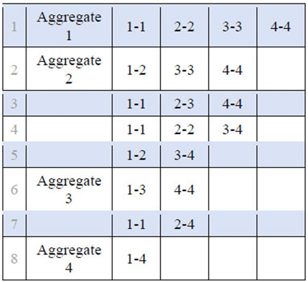
Aggregating attributes becomes more complex if two or more variables are considered at the same time. Fig. (3) shows some possible aggregations of six household types that are based on two attributes. Eight different ways of aggregations are shown here, but many more aggregations are possible. This research intends to explore all the possible aggregations across multiple attributes.

In contrast to CHAID algorithms, aggregations in this research may happen across several attributes. Within each attribute, two or more categories can be aggregated.
Table 2 lists all the attributes available for this research that were considered relevant for trip generation. The number of categories for each attribute is provided in the second column. The column ‘No. of aggregations’ lists the possible number of aggregations of categories for each attribute. The final row shows that the simple number of categories would lead to 5,040 combinations of attribute definitions. When all possible aggregations were taken into account, the number of household type definitions increased to over 67 million.
| Attribute | No. of Categories | No. of Aggregations |
|---|---|---|
| Household size | 7 | 64 |
| Number of workers | 5 | 16 |
| Income category | 12 | 2,048 |
| Auto-ownership | 4 | 8 |
| Region | 3 | 4 |
| Product | 5,040 | 67,108,864 |
In this research, all 67 million household type definitions were generated and analyzed econometrically. For every definition of household types, the number of records per household type was counted. If one household type had fewer than 30 records, this definition of household types was dismissed right away. This reduced the number of definitions of household types to be further examined from 67.1 million to 51,401.
For the remaining 51,401 definitions of household types, trip rate frequencies observed in the household travel survey were calculated. Within each definition set, between 1 and 72 household types were distinguished. 1 household type means that all the households in the survey are aggregated to one type, which obviously is not a good representation of heterogeneous travel behavior. No household type definition with more than 72 types was found, as more types would have violated the rule of having at least 30 survey records per household type. As shown below, ‘more types’ are not necessarily better, as the segmentation that best represents heterogeneity may need to aggregate some categories to keep enough survey records for emphasizing differences across other categories.
The standard deviation of the trip frequencies was calculated for each household type within a given definition set. When the standard deviation was small, the definition set was assumed to effectively represent differences in the trip-making behavior between the household types. Conversely, a comparatively large standard deviation suggested that the definition of the household type did not well represent the trip-making behavior within the individual household types. The coefficient of variance was also calculated. It was found, however, that the standard deviation and the coefficient of variance correlated closely. Therefore, only the standard deviation was used subsequently. Fig. (4) provides an example how the standard deviation of trip rates was calculated for every definition of household types.
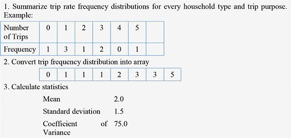
For every segmentation of household types, standard deviations were calculated. The ideal household type segmentation was selected by averaging the standard deviations of all household types. Statisticians generally advise not to calculate the average of standard deviations. Instead, variances were calculated and averaged, and the square root of their average was taken. This step generates a statistically valid average of standard deviations. Subsequently, the one household type segmentation that led to the smallest average standard deviation was selected as the one that best represented heterogeneity in trip making.
Six trip purposes were distinguished:
- Home-based work (HBW)
- Home-based shop (HBS)
- Home-based other (HBO)
- Home-based education (HBE)
- Non-home-based work (NHBW)
- Non-home-based other (NHBO)
Commonly, the same household type definition is used for every trip purposes. This research showed, however, that varying household type definitions for each trip purpose better represents differences in trip making. In a microsimulation environment, it is almost effortless to vary definitions of the household type by trip purpose, an undertaking that is computationally challenging in aggregate approaches.
Table 3 shows the household type definitions found to be ideal for every trip purpose after analyzing 51,401 possible segmentations.
| Purpose | Min No. Records per HH type | Avg. No. Records per HH type | Max No. Records per HH type | Min Std Dev | Avg. Std Dev | Max Std Dev | Min Coeff of Var | Avg. Coeff of Var | Max Coeff of Var |
|---|---|---|---|---|---|---|---|---|---|
| HBW | 48 | 598.5 | 1,936 | 0.27 | 0.45 | 2.27 | 39.60 | 32.95 | 710.64 |
| HBS | 30 | 478.8 | 2,514 | 0.86 | 0.71 | 4.07 | 112.69 | 23.15 | 175.93 |
| HBO | 30 | 478.8 | 2,514 | 1.19 | 1.06 | 6.49 | 77.16 | 18.62 | 136.78 |
| HBE | 30 | 478.8 | 2,514 | 0.06 | 0.39 | 2.97 | 74.18 | 93.68 | 1774.82 |
| NHBW | 30 | 342.0 | 1,544 | 0.11 | 0.50 | 2.01 | 100.94 | 50.74 | 1115.79 |
| NHBO | 39 | 798.1 | 3,410 | 0.85 | 0.88 | 3.31 | 122.36 | 27.50 | 233.41 |
Table 3 also shows the smallest and highest standard deviations found. It was found, however, that minimum, average and maximum standard deviations correlated closely, which is why the selection of the household type definitions could be reduced to review the average standard deviations. A small average standard deviation of the trip frequencies was taken as evidence that a given household type segmentation effectively represented the observed trip-making behavior. Table (4) shows the household type definitions for each segmentation selected in Table (3). For the HBW trip-making behavior, for example, household size was not found to be as relevant. Therefore, all seven household size categories were aggregated (indicated by “1-7” in Table (4)). The number of workers in each household, on the other hand, was identified to be highly relevant for HBW trip-making behavior, and households with 0, 1, 2, and 3+ workers were distinguished. It intuitively made sense that the number of workers was found to be much more important than the household size to estimate the number of work trips. Income was fairly relevant, particularly at the high end, which is why categories 1-5, 6-7, 8, 9-10, 11 and 12 were kept separate. Little surprising, auto ownership was not found to be relevant, as most workers needed to make work trips, regardless of auto availability. Regions (1=urban, 2=suburban and 3=rural) were not found to make a significant difference either, at least not in the case when each household type needed to be covered by at least 30 survey records.
| Trip purpose | Number of HH types | HH Size Segmentation | Worker Segmentation | Income Segmentation | Auto-ownership Segmentation | Region Segmentation |
|---|---|---|---|---|---|---|
| HBW | 24 | 1-7 | 0-0.1-1.2-2.3-4 | 1-5.6-7.8-8.9-10.11-11.12-12 | 0-3 | 1-3 |
| HBS | 30 | 1-1.2-2.3-3.4-4.5-7 | 0-4 | 1-6.7-12 | 0-1.2-2.3-3 | 1-3 |
| HBO | 30 | 1-1.2-2.3-3.4-4.5-7 | 0-4 | 1-6.7-12 | 0-1.2-2.3-3 | 1-3 |
| HBE | 30 | 1-1.2-2.3-3.4-4.5-7 | 0-4 | 1-6.7-12 | 0-1.2-2.3-3 | 1-3 |
| NHBW | 42 | 1-7 | 0-0.1-1.2-4 | 1-3.4-4.5-5.6-6.7-8.9-10.11-12 | 0-3 | 1-1.2-3 |
| NHBO | 18 | 1-1.2-2.3-7 | 0-0.1-4 | 1-12 | 0-0.1-1.2-3 | 1-3 |
For non-work trip purposes, the household size was found to be important and the number of workers turned out to be irrelevant. Auto ownership turned out to be important for all non-work trip purposes. This is in line with expectations, as many non-work trips are discretionary trips, where owning a car makes it easier to travel, and therefore, such trips are made more frequently. Region type “urban” was found to be relevant for non-work trips, where most of these trips were made. After these household types were defined, a microscopic trip generation module was developed to be compared with the existing aggregate trip generation module.
5. MICROSCOPIC TRIP-GENERATION METHOD
In this microscopic trip generation model, trips by purpose are generated individually for each household. While aggregate travel demand models commonly work with aggregated socio-economic data, the microsimulation trip-generation module requires microscopic socio-economic data.
The land use model SILO [15] was used to create a synthetic population for the study area of interest. SILO uses PUMS4 micro data and expands these data to county-level control totals. PUMS data provide all household and person attributes necessary for microscopic trip generation, including household size, household income, number of workers and auto ownership. The microscopic households can be updated for future years using the SILO land use model.

For every household, the number of trips is generated individually. The definitions of household types shown in Table 4 are used to identify the household type. Using the household travel survey, the trip frequency distribution for a given household type and a given purpose is used to randomly select the number of trips generated by this particular household. Thereby, the entire span of number of trips generated by this household type is represented. Going back to the example shown in Table (1), some households will make five trips, even though this will be a rather rare event. Most households in this example will choose to do 0, 1 or 2 work trips. In any case, the number of trips will be a discrete number, and no fractional trips (such as 1.24 trips) are created by the microscopic model. The flow diagram in Fig. (5) shows the microscopic trip generation procedure. For every household, the number of trips generated for each purpose was chosen by Monte Carlo simulation based on the observed trip rate frequencies for this household type. Instead of selecting an average number of trips for each household of the same type, some households were chosen to have unusually many trips, while others were chosen to have no trips. This diversity in trip generation is more realistic than assigning the same average number of trips to each household.
The procedure continued until trips for all households and all six trip purposes were generated. The result of this step was a long list of trips by household and by purpose. Trips may be aggregated by zone and purpose, if the subsequent modules are aggregated. However, the microscopic representation of trips allowed maintaining all the household attributes for subsequent modules. If the mode choice model needs occupation, for example, this household attribute is maintained and not eliminated, as the traditional aggregate trip generation model would do.
6. MODEL VALIDATION
To explore the impact of the microscopic trip generation module, the subsequent model steps of the MSTM (destination choice, mode choice, time-of-day choice and assignment) were run, and assigned traffic volumes were compared against count data. Table 5 compares the original and fully aggregate model with the microscopic trip generation model by purpose and income. It shows that the microscopic approach generally produced fewer low-income trips and more high-income trips. The microscopic module is more capable of representing trip making, because all 12 income categories of the survey were considered in the microscopic approach, while the aggregate trip generation module forced all trip purposes into the same five income categories. Low-income households tended to make fewer work trips than high-income households, a relationship that was underrepresented using five income categories of the aggregate approach.
| Purpose | Aggregate | Microscopic | Deviation |
|---|---|---|---|
| HBW 1 | 699,535 | 379,066 | -46% |
| HBW 2 | 1,334,802 | 942,738 | -29% |
| HBW 3 | 1,701,074 | 1,377,938 | -19% |
| HBW 4 | 1,256,971 | 2,765,313 | 120% |
| HBW 5 | 1,245,440 | 2,279,653 | 83% |
| All HBW | 6,237,822 | 7,744,709 | 24% |
| HBS 1 | 882,040 | 745,840 | -15% |
| HBS 2 | 1,294,203 | 999,123 | -23% |
| HBS 3 | 1,717,030 | 1,155,999 | -33% |
| HBS 4 | 1,215,363 | 2,130,301 | 75% |
| HBS 5 | 1,087,876 | 1,634,735 | 50% |
| All HBS | 6,196,512 | 6,665,997 | 8% |
| HBO 1 | 1,690,449 | 1,451,606 | -14% |
| HBO 2 | 2,670,943 | 2,068,263 | -23% |
| HBO 3 | 3,570,647 | 2,537,374 | -29% |
| HBO 4 | 2,350,820 | 5,519,035 | 135% |
| HBO 5 | 2,433,201 | 4,216,852 | 73% |
| All HBO | 12,716,060 | 15,793,130 | 24% |
| HBE | 1,663,393 | 1,533,004 | -8% |
| NHBW | 8,132,394 | 4,732,360 | -42% |
| NHBO | 14,334,087 | 8,033,623 | -44% |
The conclusion that the microscopic model performs better was supported by the reduction of mode-specific constants in the mode choice models. Smaller constants are desirable, as more behavioral variations are explained through the model, and less are accumulated in static constants. Reducing constants improves the overall model sensitivity. After implementation of the microscopic trip generation, the mode choice model was recalibrated, and mode-specific constants were reduced by an average of 9 percent. Fig. (6) compares mode-specific constants before (x-axis) and after (y-axis) the introduction of microscopic trip generation. The dotted line is the diagonal. Because the actual regression line (dashed line) has a smaller slope than the dotted line, constants are closer to 0 on the average after introducing microscopic trip generation.
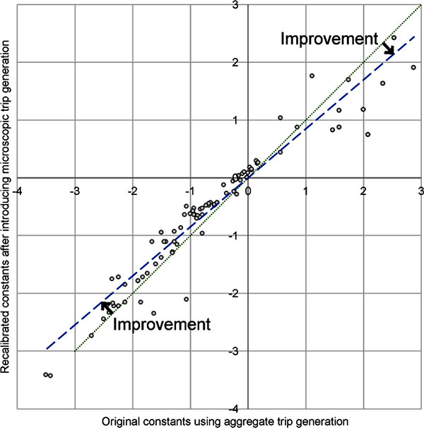
Table 6 compares validation statistics of both the aggregate and the microscopic model after assigning volumes to the network and comparing modeled volumes with the observed traffic counts. R2, Root Mean Square Error (RMSE) and the Percent RMSE were compared. Higher R2 and smaller RMSE and % RMSE show that the microscopic model setup better represents travel demand than the existing aggregate approach. The implementation of the microscopic trip generation module improved the RMSE assignment validation by 7 percent.
| Model | Deviation across all counts | R2 | RMSE | %RMSE |
|---|---|---|---|---|
| Aggregate trip generation | -2.3% | 0.888 | 7,243 | 40% |
| Microscopic trip generation | 1.4% | 0.903 | 6,764 | 38% |
| Improvement | 39% | 2% | 7% | 5% |
CONCLUSION
The microsimulation of trips offered several benefits. Foremost, the actual trip frequencies observed in the travel demand surveys were preserved. Instead of forcing every household to generate an average number of trips, which usually is a fractional number that cannot be completed by any household in reality. The observed integer number of trips were generated for every household. The variety of trip frequencies was preserved as it can be found in reality, including a few households making an uncommonly large number of trips and other households making no trips at all.
Furthermore, household types do not need to be defined identically for every trip purpose. As shown in Table (4), household size is irrelevant for work trips, but highly relevant for non-work trips. For the attribute number of workers, the opposite is true. Income turned out to be very relevant for work trips, while auto ownership did not affect these trips. The distinction of regions (urban, suburban and rural) only turned out to be relevant for non home based work trips, for which the urban region received a different trip generation frequency than suburban and rural areas. This nicely aligns with the observation that most non home based work trips are observed in the urban centers where most jobs can be found.
Furthermore, mode-specific constants were reduced and the assignment result improved. Maybe the most important benefit, however, is that all the attributes of the synthetic population were preserved through trip generation. This opens large opportunities for destination choice, as now auto-availability, occupation, income, and many other socio demographic attributes can be considered to select destinations. Moreno and Moeckel [16] explored the potential improvements to be made in the destination choice model. One of the biggest advantages of retaining microscopic data is their flexibility to be aggregated in any way needed for the purpose at hand [17].
A limitation of this approach is that travel behavior is still represented in trips and not in activities that result in tour generation. Activity based models [18] care for the actual purpose of making a trip (that is doing an activity). By individually representing travelers, activity based models usually create tours rather than single trips. In aggregate 4-step models, tours are represented less thoroughly by introducing non-home-based trips. However, implementing an activity based model is a significant undertaking. This paper described an approach that enables users of 4-step models to gain one of the most compelling aspects of activity-based models, namely the microsimulation framework itself, without the huge cost of moving to one. Microsimulation enabled this approach to add more variables, which improved the model’s accuracy and (perhaps more importantly) policy sensitivity.
Another benefit of adding a microscopic trip generation module to an existing 4-step model is to maintain an operational model while improvements are under development. This development paradigm pursued in this study is called agile development in computer science [19]. In agile approaches, single modules are updated while an operational model is preserved at any time. Resources are focused on modules that deserve most attention for improvements. Agile model development promises to implement advanced models while keeping an existing model operational. Fig. (7) shows the vision of this development path for this model.
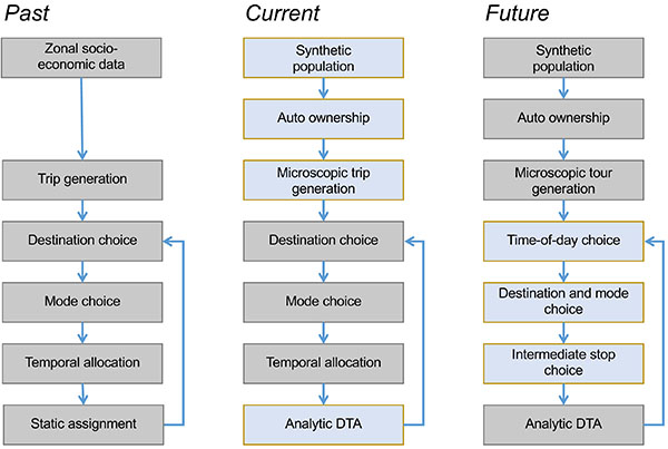
Following this envisioned path, it is planned in the near future to add a microscopic time-of-day choice model and a microscopic destination choice model. Moving towards microscopic models may affect the runtime. The creation of the synthetic population takes approximately 30 minutes. Given that this runs only once, the additional runtime is not as relevant. The auto-ownership model and the microscopic trip generation model run within 3 minutes, and therefore, do not add significantly to the model’s runtime compared to the aggregate version. The Analytic DTA, however, has increased the runtime substantially from 5 hours for the static assignment to 16 hours for the Analytic DTA. Such increases in the runtime need to be considered carefully against the capabilities of the improved model. Currently, both the static assignment and the Analytic DTA are kept in parallel, and the latter is only used for scenarios for which DTA matters. The agile development approach allows reviewing runtimes after each model improvement, and future model development can be adjusted accordingly.
A side benefit of modeling destination choice microscopically will be to preserve the regular workplace defined in the synthetic population. In traditional aggregate models, in which the workplace is newly chosen every iteration, different travel times trigger households to choose a new workplace instantaneously. Obviously, this behavior is rather unrealistic. Furthermore, aggregate models are unable to consider a household’s travel budget, both in terms of time and money. Zahavi [20] suggested and Schafer [21] later confirmed that the travel budgets at the aggregate are fairly constant and change at most slowly over time. Trip-based models, however, by definition do not take into account travel budgets. If congestion worsens, trip-based models will trigger households to spend more time on traveling, which is a violation of Zahavi’s paradigm. A microscopic destination choice model can be used to ensure that average travel budgets are taken into account, both temporally and monetarily. Microscopic trip generation is the first step to move aggregate models towards this goal.
NOTES
1 Source: 2007/2008 TPB Household Travel Survey for the Baltimore/Washington region
2 Income groups are defined as <$20,000; $20,000 to $39,999; $40,000 to $59,999; $60,000 to $99,999; $100,000 or more
3 Income categories are defined as Less than $10,000; $10,000 - $14,999; $15,000 - $29,999; $30,000 - $39,999; $40,000 - $49,999; $50,000 - $59,999; $60,000 - $74,999; $75,000 - $99,999; $100,000 - $124,999;$125,000 - $149,999; $150,000 - $199,999; $200,000 or more
4 Public Use Micro Data (PUMS) are anonymized microscopic census data of individual households and their household members, available for download at http://www.census.gov/acs/www/data_documentation/ public_use_microdata_sample/
FUNDING DETAILS
The research was completed with the support of the Technical University of Munich – Institute for Advanced Study, funded by the German Excellence Initiative and the European Union Seventh Framework Program under grant agreement n° 291763. In part, this research was also funded by the Maryland State Highway Administration.
CONFLICT OF INTEREST
The authors confirm that this article content has no conflict of interest.
ACKNOWLEDGEMENTS
Declared none.

