The Trolley Problem Version of Autonomous Vehicles

1. INTRODUCTION

Ethics is not an exact science. Someone can consider one decision as moral; whereas the other one can consider the very same decision as immoral. When it comes to autonomous vehicles, the ethics should be sometimes encoded into the software of the vehicle. The programmer should sometimes decide questions like whose life is more precious, the occupants in the vehicle or pedestrians go nearby the vehicle?

Such questions have been weighed up over the years and specifically for autonomous vehicles in the recent years [1], but no clear decisions have been made. One of the most popular forms to present the question about the priority of human lives is the “Trolley Problem” [2]. There are some versions for the trolley problem but the common concept is that there is a need to prioritize the life of several persons.

In the “Trolley Problem” the situation is clear i.e. you should kill a certain person in order to save another certain person; however, the reality is not so clear [3, 4]. Sometimes the software of the autonomous vehicle cannot be sure whether in a case of an accident, the occupants in the vehicle, nearby pedestrians or anyone else will die. e.g. when there is a rollover crash the occupants in the vehicle have a smaller chance to die relative to a pedestrian that the vehicle falls on him; however, there is still a small chance that an occupant in the vehicles will sustain a severer injuries than a nearby pedestrian [5].

There was a claim that the autonomous vehicle makers prefer the lives of the occupants in the autonomous vehicle over the lives of the pedestrians in their surroundings, because the occupants are their customers and the vehicle makers

want to please them and convince more potential customers that the vehicle is safe [6]; however, no evidence has been found for this hypothetical claim [7].

This paper suggests a way to give the most accurate data to the algorithm and according to this data, the software can decide whatever decision the software developer believes is the most appropriate one.

2. METHODS

Polygons are simple shapes that can simulate the real objects. It is very common to generate models of real objects using simple polygons. This practice is usually called Spatial Data Structures [8].

When it comes to simulation of car accidents, Spatial Data Structures are implemented in order to find the intersections between two objects that are about to collide and realize which polygons are about to be damaged. Obviously, trying to check all the polygons of each of the objects is pointless, because there are parts of objects that have no chance to collide with another object in some sorts of crashes, for e.g. in a front accident, the rear part of the vehicle will not be damaged; therefore, there are several methods to reduce the number of polygons intersections when using Spatial Data Structures [9].

Spatial Data Structures are the basis for Space Partitioning [10] and Bounding Volumes [11]. Space Partitioning is a method of space sub-partitioning into convex regions. These convex regions are named “cells”. Each of these cells maintains a list of objects that it comprises of. By employing these cells, the intersection algorithm knows how to sift out pairs of polygons that have no chance to intersect.

The other method is Bounding Volume. This method breaks an object into small components; then the algorithm finds a fitted bounding volume for each of the small component. After that, the intersection algorithm checks for intersected components. It should be noted that the sifting out is less demanding in this method, because the algorithm just have to detect the at least partly cover bounding volumes.

Bounding Volumes applications have been intensely studied over the years and many variations of the method have been suggested: Bounding Spheres [12], K-DOPs - Discrete Orientation Polytopes [13], OBB - Oriented Bounding Boxes [14], AABB - Axis Aligned Bounding Boxes [15] and Hierarchical Spherical Distance Fields [16].

In this paper, we have used the AABB approach which is one of the most well-known approaches. In AABB, each of the bounding volume in the object model is represented by its minimum and its maximum values. Compared to the “Bounding Sphere” approach, AABB has an advantage and a disadvantage. AABB encompasses the components of the model more tightly which probably yield fewer intersection checks and also the split of the object into its bounding volumes is faster [17]. The algorithm first checks each of the basic elements that a bounding volume consists of and projects the element on the axes and then finds the minimum and the maximum values for each axis. The fast operation is quite essential in real-time systems like collisions of autonomous vehicles. The algorithm should be fast and decide promptly what course of actions should be taken.

However, AABB also has a disadvantage. Saving the data for AABB takes more memory space which in the past was very costly, but nowadays, ample memory space is quite economical and even simple computers have plenty of memory space, so this disadvantage is not so acute; therefore, we have chosen the AABB approach.

Since our system is a real-time system and the computation time is very essential we have decided to implement the AABB approach. We generated the bounding volume tree in a recursive manner. In each step, the algorithm generates bounding volumes for the remaining triangles and splits the triangle set into two sub-graphs. Then, it recursively calls itself to do the same for each of these sub-graphs.

2.2. Implementation

As was explained above, the implementation of the method was in a recursive manner. We used triangles as it is a very common in such implementations [19].

Initially, the algorithm finds a bounding volume for the remaining triangles. Then, the algorithm splits the set of triangles into two sub-graphs. Finally, the algorithm calls itself in a recursive manner to handle the two new sub-graphs that have been generated in the previous step. When a sub-graph has just one triangle, the recursive call will stop and the algorithm will not call itself any longer.

The incentive for the triangles split into several sub-graphs is the formation of as small as possible bounding volumes so the model will as accurate as possible.

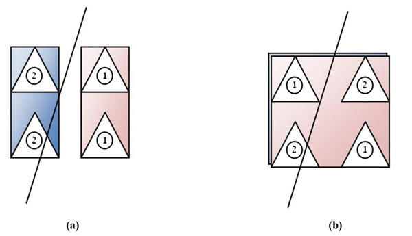
(Fig. 1a and b) explains by an example how four triangles can be split in two different ways. The number written in the triangles denotes which sub-graph contains the triangle after the suggested split. This figure clearly shows that a hierarchical intersection checking with a specific segment can generate more triangle intersection checks in the right side figure because the generated bounding volume is bigger. This attribute motivated us to implement a split algorithm that uses better splits as in the left side, so as to minimize the triangle intersection checks.

Actually, the bounding volume algorithms and the triangle split algorithms greatly shape the bounding volume tree generation algorithm and its efficiency. We have employed “Fitting points with Gaussian distribution” [20] to as the basis for the algorithm for generating the bounding volumes.

2.3. Triangle Split Algorithm

Each graph of triangles has a corresponding bounding volume that can be split into two sub-graphs. The pseudo code of this split algorithm is:

• For each axis of any volume select a positive direction.
• For each triangle find a vertex with the highest value on the projected axis.
• Sort the triangles vector by their vertex values.
• For each triangle in the triangles vector compute the sum of the projection lengths on the axis divided by the original graph projection lengths of the two sub-graphs and split this triangle in order to get a smaller sub-graphs.

The algorithm strives to do its best in order to generate the least possible intersecting sub-graphs.

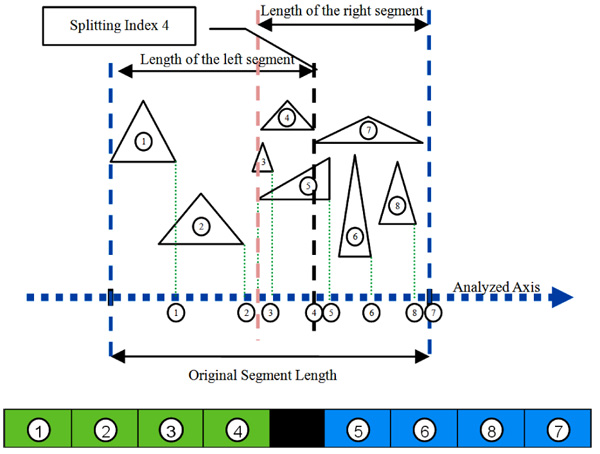
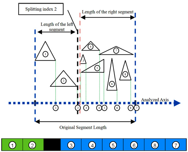
(Figs. 2 and 3) illustrate two different potential index split. (Fig. 2) shows one potential split at triangle index 4. If indeed the algorithm chooses to split at this index, the split will ineffectually generate a larger intersection between the two new graphs. (Fig. 3) shows a better option which is a split in triangle index 2 which generates a smaller intersection between the two new graphs. This example shows a case when the algorithm would select a better split over an inferior split. In this particular example, it was a split at triangle index 2 rather than a split at triangle index 4.

4. RESULT

We evaluated several schemes for parallel implementation of the algorithm:

• Best Match – Select a core with the maximum number of correlated model sections.
• Random Match – Select a random core.
• Lowest Match - Select a core with the minimum number of correlated model sections.
• Best Match-Load – This is a combination of the Best Match scheme and a Load parameter that calculated for each core. The algorithm prefers less loaded cores over more loaded cores. The load on any core is computed by dividing the buffered checks waiting for this core by the maximal size of this core's buffer. The algorithm takes into account both the load in the core and the correlation between the model sections that the core checks and the newly designed model section, so as to get the best decision.

The suggested method has been implemented on a four cores processor. We endeavored to evaluate the efficiency of the suggested triangle scheme. The particular processor was Intel^® Pentium^® Processor N3540 which is a very widespread quad-core processor with 2.16GZ; however, another process would have yield similar results.

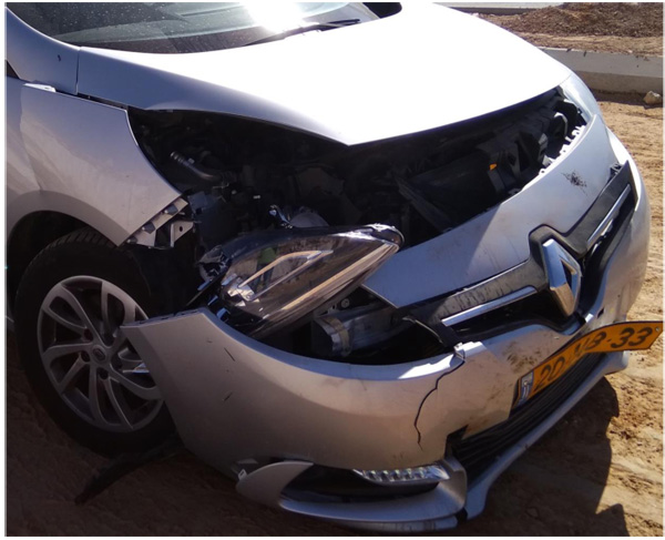
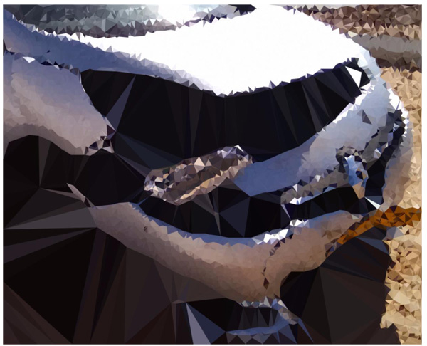
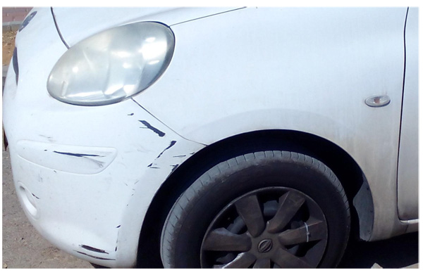
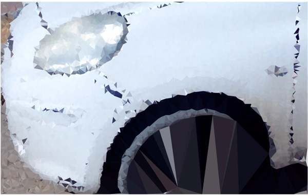
We checked two kinds of damages. In (Figs. 4 and 5), we can see a vehicle with a substantial damage. (Fig. 4) shows the vehicle before it has been triangulated and (Fig. 5) shows the same vehicle before it has been triangulated. Similarly, (Figs. 6 and 7) show a vehicle before it has been triangulated and after before it has been triangulated. However, (Figs. 6 and 7) show a vehicle with only scratches.

Selecting the distribution depth of the bounding volumes is also very important and should be carefully selected. Small depths result in large overlapping bounding volumes, which will generate many node collision pairs. However, large depths result in a long analysis of the first step by the main process, while the other cores are idle. This is an unnecessary bottleneck that the algorithm should prevent.

We have checked the effect of several distribution depths on the algorithm performance. We have used the images of the vehicle in (Fig. 5) and the vehicle in (Fig. 7). The findings can be seen in (Figs. 8 and 9). It can be noticeably observed that the Best Match algorithm yields better performance, both in relative data transfer and speedup.

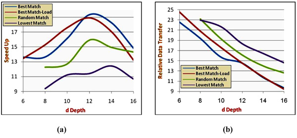
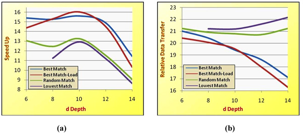
The best possible distribution depth can be different in different cases. An example of this difference can be seen in (Figs. 8 and 9). The vehicle in (Fig. 8) has an optimal distribution depth of 12; whereas the vehicle in (Fig. 9) has an optimal distribution depth of 10. Other vehicles can have other optimal distribution depths.

5. DISCUSSION

The results clearly show that different distribution depths should be chosen for different vehicle models.

Moreover, we can also figure out from the results that if the vehicle model is larger, the Best Match algorithm will have a greater benefit over the other algorithms.

The buffer size of the cores has a noticeable effect on the performance of the algorithms. The buffer gives a core option of collecting several jobs and sending them en masse to another core. Therefore, the main process has more time for setting up tasks for other cores.

If we choose an algorithm that consumes more memory, like Lowest Match or Random Match, the processor will swiftly run out of memory and therefore will be incapable to accomplish the task. The processor will have to bring into play virtual memory mechanism that can turn out even to thrashing [21].

Such a situation can be seen in the last Figures where there are trimmed lines. It occurs in algorithms that inefficiently allocate memory and when a low distribution depth is select. The lines are trimmed because the algorithm went into a thrashing situation and therefore no data could be obtained.

CONCLUSION

There is no confident moral answer to the “Trolley Problem” and different people gave different moral answers to this problem. Our paper also did not aim at realizing the “correct moral answer” for the “Trolley Problem” and it was out of scope of this paper. The aim of this paper is to emphasize that the “Trolley Problem” occurs when the human driver is replaced by a robot and if a moral answer is given by an authoritative and legitimate board of experts, it can be coded in autonomous vehicle software.

The paper has suggested a real-time estimation system for vehicle crash probable damages. The aim of this system is to facilitate autonomous vehicle's embedded computer to decide which crash is the least harmful when it comprehends that a crash is unavoidable by analyzing all the damaged for each of the possible crashes.

Actually, this paper has suggested how to adapt the well-known Primitive Intersection scheme into an estimation tool of potential vehicle crash damages so as to decide which course of actions should be taken by the vehicle in an inescapable crash.

In the future, we consider checking how other strategies could be implemented and also the advisability of using other polygonal shapes.

REFERENCES