All published articles of this journal are available on ScienceDirect.

The Analysis of Dynamic O/D Adjustment for Bicycle Traffic Demand Estimation with AIMSUN Simulation Model: A Case Study of Nakhon Sawan Municipality in Thailand
Abstract
Aim:
This research aimed to present the process of estimating bicycle traffic demand in order to design bike routes that meet the daily transportation needs of the people in Nakhon Sawan Municipality.
Methods:
The primary and secondary traffic data were collected to develop a virtual traffic simulation model with the use of the AIMSUN simulation software. The model validation method was carried out to adjust the origin and destination survey data (O/D matrix) by running dynamic O/D adjustment. The 99 replication scenarios were statistically examined and assessed using the goodness-of-fit test. The 9 measures, which were examined, included: 1) Root Mean Square Error (RMSE), 2) Root Mean Square Percentage Error (RMSPE%), 3) Mean Absolute Deviation (MAD), 4) Mean Bias Error (MBE), 5) Mean Percentage Error (MPE%), 6) Mean Absolute Percentage Error (MAPE%), 7) Coefficient of Determination (R2), 8) GEH Statistic (GEH), and 9) Thiel’s U Statistic (Theil’s U).
Results:
The resulting statistical values were used to determine the acceptable ranges according to the acceptable indicators of each factor.
Conclusion:
It was found that there were only 8 scenarios that met the evaluation criteria. The selection and ranking process was consequently carried out using the multi-factor scoring method, which could eliminate errors that might arise from applying only one goodness-of-fit test measure.
1. INTRODUCTION
The Thai government has placed importance on formulating policies to solve traffic congestion in a sustainable way. INRIX [1] assessed traffic conditions in 195 countries and revealed that in 2017 Thai drivers spent an average of 56 hours in traffic congestion during peak hours, compared to 61 hours in 2016. Although its traffic congestion was getting less over the two years, Thailand was still ranked the most traffic-congested country, out of 38 countries with the worst traffic in the world. Thus, the government has tried to solve the problem by launching an emergency plan to promote changes in the mode of transportation in every province of Thailand. The people that need to commute to areas within a 20 kilometer radius from their house are encouraged to use bicycles instead of private cars. However, there are still problems in the current bike route design because most bike routes were mainly designed based on the preferences of designers and existing cyclists, which sometimes might not cover the traffic demand of people in each community. This made private car drivers unwilling to change their transportation mode or use bicycles for daily transportation. After reviewing the results of bike route evaluation in many areas, it was found that the number of bike route users was lower than expected, the budget was not invested in worthwhile projects, and the design failures often caused traffic accidents [2].
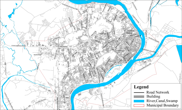
Nakhon Sawan Municipality is one of the first cities in Thailand that seriously promote the use of bicycles. It is located in the central region, where the Ping and Nan Rivers converge and form the Chao Phraya River, the most important waterway of Thailand, as shown in Fig. (1). Its population density is 3,010 people per square kilometer [3]. Nakhon Sawan Municipality is considered one of the largest cities in Thailand.
Nakhon Sawan Municipality built the first bike route around Sawan Park for exercise purposes in 2013 [4]. Then there was an initiative to extend and develop that bike route into the community’s daily transportation network. The qualitative research was conducted using focus group discussions. The four groups of informants, consisting of 1) government officials, 2) designers, 3) users, and 4) press, were selected to share their opinions about bike routes. The results suggested that a circular bike route should be designed along the main roads and a shared bikeway should be built separately from the main traffic lane [2]. However, the results of that research only reflected the traffic demands of 4 groups of people. The daily traffic demand of other groups of people had not been examined. Therefore, the present research aimed to analyze the estimated traffic demand in the road network of Nakhon Sawan Municipality with the use of the AIMSUN simulation program. The model validation method was also carried out to adjust the origin and destination survey data according to the traffic engineering principles. This is to ensure that the resulting data can be used to effectively design the bike route network that truly meets the community’s daily traffic demand.
This paper is organized as follows. Section 2 introduces the statement of problem. Section 3 presents the review of the literature. Section 4 describes how to survey data and generate an AIMSUN simulation model as well as explains the implementation of data analysis and model validation processes. Section 5 shows the results of running 99 replication scenarios of dynamic O/D adjustment, the results of statistical analysis, the acceptable deviation criteria, and the application of the multi-factor scoring method to the selection and ranking of O/D matrix adjustment. Sections 6 gives summary and conclusion of the present study.
2. STATEMENT OF PROBLEM
As the main transportation mode in Nakhon Sawan Municipality is private cars, it is important to analyze the traffic demand of private car users between origin and destination sub-areas and use the obtained results to design a bike route that meets the daily transportation needs. This will help motivate local people to use bicycles as their main transportation mode instead of private cars. According to the traffic engineering principles, the origin and destination survey can be carried out in many different ways through the use of questionnaire technique [5], license plate matching technique [6-9], or Bluetooth MAC address readers [10]. The present research used the license plate matching technique to conduct the origin and destination survey because it is the most common method that requires less budget and can be easily applied to other areas in Thailand. However, the results of the license plate matching in each checkpoint indicated that there are only a few matching entries, compared to the traffic volume during the survey period. The road network of Nakhon Sawan Municipality and other cities in Thailand is not systematically organized according to the road functional classification and hierarchy of movement [11], causing each sub-area to have multiple access routes. Thus, conducting a survey that covers all traffic routes is difficult and requires a large budget.
3. LITERATURE REVIEW
Traffic simulation is considered an important tool in traffic engineering. It is used to analyze and test the design or concept of research, which helps reduce cost and impact that may occur when compared to field test. Most research studies on traffic simulation model are associated with analyzing traffic behaviors and evaluating the design or improvement of the physical characteristics of roads.
Tran Vu Tu and Kazushi Sano [12] conducted an analysis of the impacts of scramble crossings in comparison with traditional crossings on the intersection performance by using the Paramics simulation model. John Sangster et al. [13] examined the operational aspects of the through-about intersection design and carried out the comparative analysis of overall intersection delays using the SYNCHRO traffic software. Lenorzer A. et al. [14] used the Aimsun micro simulator to evaluate new road design solutions through developing a new mixed-flow model, which aimed at providing a detailed and robust behavioral data and simulating sensitivity analysis that focused on the capacity and jam density as well as the application to busy junctions in a city [14]. David Stanek [15] also studied the increased use of cycle tracks that leads to investigations of how to accommodate them at the intersection by using the VISSIM traffic analysis software. In addition, there are research studies on bicycle traffic simulation that are involved with the management of bike sharing systems. For example, Thibaut Dubernet and Kay W. Axhausen [16] developed the multi-agent activity-based simulation model to estimate the reactions of the demand to changes in the quality of the bike redistribution and relocation strategies. Robert M. Saltzman and Richard M. Bradford [17] investigated an appropriate number of docks and bikes to reduce operators’ time and resources (including fossil fuels) in moving bikes from stations with an excess of bikes to those with shortages by using an animated discrete-event simulation model.
There are some studies that propose the procedures of model construction, calibration, and validation in order to ensure the accuracy and credibility of each virtual traffic model. For example, Oketch T. and Carrick M [18]. suggested that the calibration effort involved comparing the model results to the field data that included traffic volume, movement, average travel time, and approach queues. Paramics uses a dynamic assignment procedure in which movements of vehicles through the network are governed by origin-destination matrices on the basis of various assignment techniques. The modeling exercise involved estimation of suitable origin-destination matrices which could replicate the observed traffic volumes and turning movement counts at selected intersections to acceptable levels. In addition, Chen-Ju Wu et al. [19] developed A procedure for constructing and calibrating a microsimulation model of a congested freeway with multiple vehicle classes by using AMSUN microsimulation model. They also suggested that the model construction and calibration procedure is composed of the following steps: 1) building the road geometry in AIMSUN, 2) collection of the traffic condition data from the PeMS database, 3) imputation of missing data, 4) estimation of on-ramp demand and off-ramp turning, 5) identification of recurring bottlenecks, 6) setting model parameters, and 7) adjustment of model parameters such that the simulation results match with the field measurements.
As the accuracy of the model is very important, the process of model validation is carried out in order to examine, assess, compare, and explore the relationships between observed traffic volume and modelled count data. According to the general simulation literature, a simulation model can be statistically validated using a goodness-of-fit test. UK Highways Agency [20], AIMSUN [21] and Xiao-Yun Lu et al. [22] indicated that two alternative analytic methods that are frequently applied to validation comparisons are: 1) the GEH statistic, which is a form of the Chi-squared statistic that incorporates both relative and absolute errors, and 2) the R Squared (R2), which gives some measure of the goodness of model fit and the slope of the best fit regression line. Theil H [23]. proposed the Theil’s U statistic measure that forecasts accuracy by comparing two auto-correlated time series with predicted values and observed values [23]. Tomer Toledo and Haris N. Koutsopoulod [24] stated that Among a number of goodness of fit measures, the Root Mean Square Error (RMSE), the Root Mean Square Percentage Error (RMSPE%), the Mean Error (ME), the Mean Percentage Error (MPE%), and the Thiel’s U measure (Theil’s U) are the popular ones. Daiheng Ni et al. [25] also proposed Additional goodness of fit measures, which are the Mean Absolute Error (MAE) and the Mean Squared Error (MSE). Jonathan Annan et al. [26] suggested that the Mean Absolute Deviation (MAD) is an effective measure of the average of the absolute difference between the actual observations and the predicted variable in the time series.
However, the process of model validation can be conducted using different goodness-of-fit test measures. In each research study, only a few measures are used to analyze and describe the validity of traffic simulation model. Based on this knowledge gap, the present research aimed to study the application of AIMSUN simulation model in estimating traffic demand. Nine goodness-of-fit test measures were selected to use in the model validation process. A procedure of model calibration and validation relating to statistical measurement was developed. Then the scenario with the highest score, resulting from running 99 replication scenarios of dynamic O/D, was selected using the multi-factor scoring method. The multi-factor scoring method is a collection of quantitative methodologies that can be used to make a choice from a set of alternatives by using a set of two or more factors as decision choice criteria [27]. This method has been widely used to prioritize and gives support to the management of project portfolios [28]. It is also used to evaluate and select early stage technology and innovation the projects during the decision-making process [29].
4. RESEARCH METHODOLOGY
4.1. Research Procedures
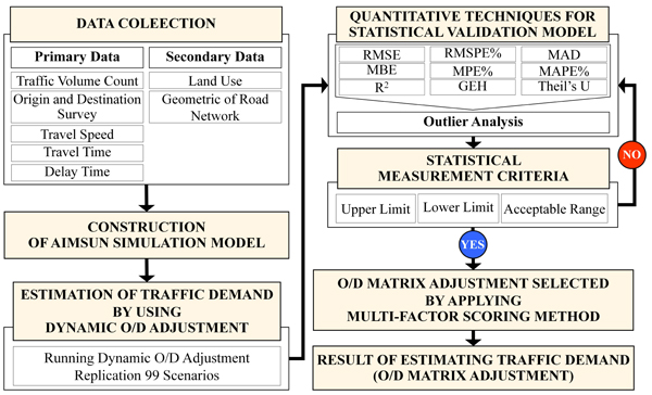
The process of traffic demand estimation was comprised of the following 7 steps: 1) collecting data, 2) developing AIMSUN simulation model, 3) estimating traffic demand by using dynamic O/D adjustment, 4) using quantitative techniques to statistically validate the model, 5) creating statistical measurement criteria, 6) applying the multi-factor scoring method to carry out O/D matrix selection and adjustment, and 7) obtaining the results of traffic demand estimation. The details are shown in Fig. (2).
4.2. Field Data Collection
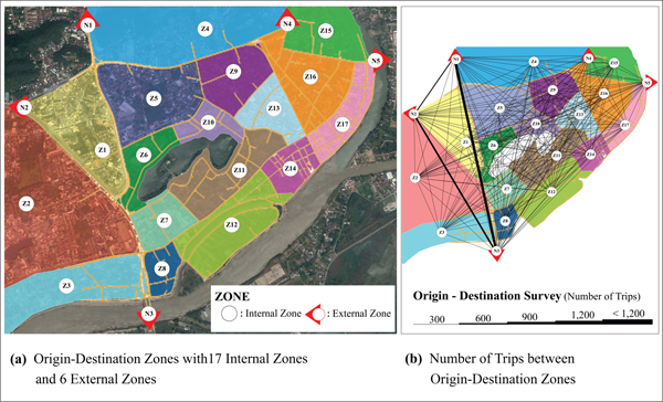
The traffic field survey was carried out to collect the data about functional classification and geometric design of road network, traffic volume, travel speed, travel time, delay time, traffic management, and origin-destination trips [11, 30, 31]. The data about traffic behavior related to the campaign that encouraged people to change their daily transport mode from private car to bicycle were collected on weekends during 6:00 AM - 1:00 PM [2]. In terms of traffic volume, the mid-block counts were conducted in 15-minute intervals at 54 locations and the vehicles were categorized into 8 groups. The observed traffic volume was subsequently converted into Passenger Car Unit (PCU) before importing to database in form of Real Data Sets (ISO Format YYYY-MM-DDTHH:MM:SS). The origin-destination survey was carried out in 18 locations with the license plate matching techniques [6-9] in order to examine the traffic demand in Nakhon Sawan Municipality that were classified into 23 sub-areas (17 internal sub-areas and 6 external sub-areas) according to land use purposes [30]. The survey results are shown in Fig. (3). The data about travel speed, travel time, and delay time were collected using the test vehicle techniques [32]. The Global Positioning System (GPS) and GPS car video recorder were installed to record traffic movements and display all related information while driving through the roads [33].
4.3. AIMSUN Simulation Model
AIMSUN is a traffic simulator that follows a microscopic simulation approach. The behavior of each vehicle in the network is continuously modelled throughout the simulation time period while it travelled through the traffic network, according to several vehicle behavior models such as car following and lane changing. The input data required by AIMSUN dynamic simulator is a simulation scenario. The simulation parameters are fixed values that describe the experiment and some variable parameters used to calibrate the models [21]. In order to improve the accuracy of model, the O/D matrix data should be adjusted to observe traffic volume (Real Data Sets). The O/D matrix adjustment can be carried out by combining direct and indirect model estimators with other aggregated information related to O/D demand flows [34, 35]. The O/D matrix adjustment is based on a bi-level model solved heuristically by a gradient algorithm. It is a procedure for estimating an O/D matrix, from an a priori O/D matrix, using link traffic counts for which observed traffic volume (Real Data Sets) is available [36].
4.4. Construction of the AIMSUN Simulation Model
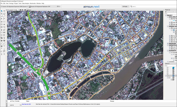
A 1:4,000 scale aerial photograph was imported into the ArcGIS program to create GIS road network map. Then the road network was digitized and the physical characteristics of the roads were recorded and linked to attribute data such as road (Link), junction (Node), number of lane, and lane width [37]. After that, all the data were imported to create AIMSUN simulation model of the road network. Lastly, other traffic data, both primary and secondary, were separately inputted in each segment of road such as hierarchy of road, capacity, traffic variables, flows speeds, traffic management, driver behavior, and reaction time. The details are shown in Fig. (4).
4.5. Data Analysis and Validation Model
Considering the traffic demand adjustment, the results of the origin and destination (O/D) survey in form of O/D matrix were adjusted by running the dynamic O/D adjustment. The maximum number of iterations was set to 99 scenarios. The adjustment result of each scenario was clearly displayed in the O/D matrix adjustment process. Then the model validation process was carried out. All 99 scenarios were examined and evaluated using quantitative methods, which helped quantify the difference between the observed traffic volume (Real Data Sets) and the modelled count data. Quantitative validation can be performed with the use of statistical measurement. The general simulation literature includes a large number of approaches for the statistical validation of simulation models. The goodness-of-fit test was selected to use in the present research. The 9 measures that were used to quantify the model predictive accuracy consisted of 1) Root Mean Square Error (RMSE), 2) Root Mean Square Percentage Error (RMSPE%), 3) Mean Absolute Deviation (MAD), 4) Mean Bias Error (MBE), 5) Mean Percentage Error (MPE%), 6) Mean Absolute Percentage Error (MAPE%), 7) Coefficient of Determination (R2), 8) GEH Statistic (GEH), and 9) Thiel’s U Statistic (Theil’s U). Suppose there are two processes Yi (observed traffic volume) and Xi (modelled count data): Y1, Y2, …, Yn and X1, X2, …, Xn, where n is the sample size. The description of each factor is listed in Table 1. The results were analyzed using the multi-factor scoring method. The O/D matrix adjustment output of the scenario with the highest score was set as the estimated traffic demand between sub-areas in Nakhon Sawan Municipality.
| No. | Factor | Formula | Acceptable Indicators |
|---|---|---|---|
| 1 | Root Mean Square Error (RMSE) |
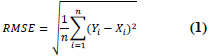 |
RMSE = 0 implies perfect fit. |
| 2 | Root Mean Square Percentage Error (RMSPE%) |
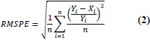 |
RMSPE% = 0 implies perfect fit. Note: The percentage error cannot exceed 100% |
| 3 | Mean Absolute Deviation (MAD) |
 |
MAD = 0 implies perfect fit. |
| 4 | Mean Bias Error (MBE) |
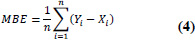 |
MBE < 0 = modelled count data is less than observed traffic volume, and MBE > 0 = modelled count data is more than observed traffic volume. |
| 5 | Mean Percentage Error (MPE%) |
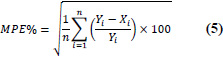 |
-10% < MPW < 10% = acceptability ranges. |
| 6 | Mean Absolute Percentage Error (MAPE%) |
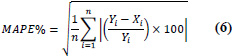 |
MAPE% = 0 implies perfect fit. Note: The percentage error cannot exceed 100% |
| 7 | Coefficient of Determination (R2) |
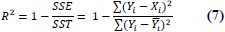 |
R2 is bounded, 0 ≤ R2 ≤ 1 R2 = 0 implies worst possible fit, and R2 = 1 implies perfect fit. |
| 8 | The GEH Statistic (GEH) |
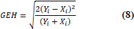 |
GEH < 5 = flows can be considered a good fit, 5 < GEH < 10 = flows may require further investigation, and 10 > GEH = flows cannot be considered to be a good fit. |
| 9 | Thiel’s U Statistic: URFORM (Theil’s U) |
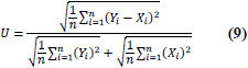 |
U is bounded, 0 ≤ U ≤ 1 U = 0 implies perfect fit, and U = 1 implies worst possible fit. |
5. ANALYSIS OF THE RESULT
5.1. Estimation of Traffic Demand by Using Dynamic O/D Adjustment
In order to simulate traffic situations, the origin-destination survey data during peak hours were imported into Demand Data in form of O/D matrix. The types of vehicles were also converted into Passenger Car Unit (PCU). The normal distribution was given for global arrivals. Then the traffic demand estimation was carried out by running dynamic O/D adjustment replication. The maximum number of iterations was set to 99 scenarios in order to find the O/D matrix adjustment output. Dynamic O/D adjustment is a procedure for adjusting a priori O/D matrix using traffic counts. It is used to adjust O/D matrix derived from demand predictions to agree with traffic volume observed (Real Data Sets, ISO Format YYYY-MM-DDTHH: MM:SS). The results and comparison of the O/D matrix adjustment of 99 scenarios are shown in Table 2 and Fig. (5).
| No. |
Road Segment (Object) |
Real Data Set (PCU/hour) |
Scenario - Dynamic O/D Adjustment (PCU/hour) | ||||||||||||
|---|---|---|---|---|---|---|---|---|---|---|---|---|---|---|---|
| 1 | 2 | 3 | 4 | 5 | 6 | . . . . | 94 | 95 | 96 | 97 | 98 | 99 | |||
| 1 | 5335:27:00 | 270 | 238 | 242 | 269 | 255 | 249 | 260 | . . . . | 260 | 261 | 261 | 275 | 230 | 262 |
| 2 | 5334: 27OUT | 211 | 253 | 246 | 240 | 203 | 217 | 226 | . . . . | 156 | 162 | 162 | 176 | 203 | 169 |
| 3 | 4291: 1OUT | 48 | 46 | 49 | 49 | 52 | 39 | 33 | . . . . | 50 | 44 | 44 | 40 | 46 | 48 |
| 4 | 4290:01:00 | 45 | 45 | 38 | 48 | 33 | 38 | 40 | . . . . | 53 | 54 | 54 | 52 | 45 | 52 |
| 5 | 4148: 54OUT | 88 | 87 | 86 | 90 | 84 | 87 | 92 | . . . . | 90 | 90 | 90 | 87 | 86 | 90 |
| 6 | 5335:27:00 | 270 | 238 | 242 | 269 | 255 | 249 | 260 | . . . . | 437 | 437 | 437 | 434 | 446 | 437 |
|
. . . |
. . . |
. . . |
. . . |
. . . |
. . . |
. . . |
. . . |
. . . |
. . . |
. . . |
. . . |
. . . |
. . . |
. . . |
. . . |
| 96 | 3838:05:00 | 192 | 217 | 190 | 194 | 203 | 208 | 201 | . . . . | 185 | 203 | 203 | 195 | 207 | 187 |
| 97 | 3835: 4OUT | 16 | 19 | 17 | 31 | 25 | 31 | 31 | . . . . | 35 | 38 | 38 | 41 | 40 | 41 |
| 98 | 3834:04:00 | 35 | 20 | 22 | 22 | 26 | 23 | 18 | . . . . | 32 | 35 | 35 | 39 | 41 | 40 |
| 99 | 3833:03:00 | 693 | 786 | 711 | 774 | 730 | 728 | 745 | . . . . | 713 | 690 | 690 | 685 | 718 | 680 |
| 100 | 3832: 2OUT | 13 | 7 | 12 | 14 | 12 | 14 | 17 | . . . . | 25 | 23 | 23 | 21 | 23 | 20 |
| 101 | 3831:02:00 | 13 | 4 | 5 | 9 | 10 | 9 | 9 | . . . . | 9 | 10 | 10 | 10 | 17 | 11 |
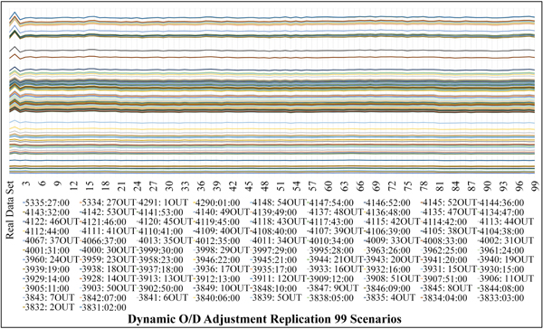
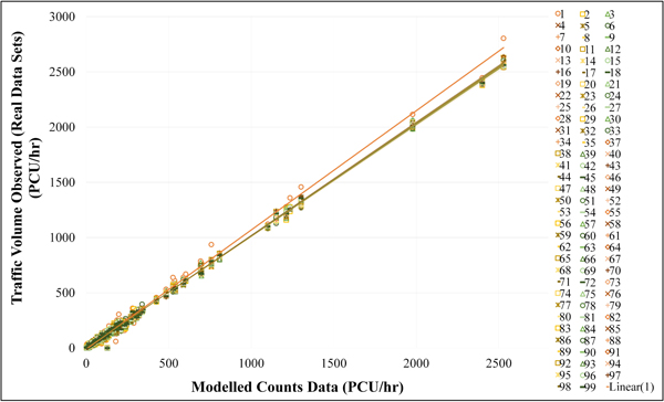
Fig. (5) shows that Scenario 1 and Scenario 2 have a similar graph pattern in each road segment (Object). The road segments with high traffic volume from modelled count data are obviously reflected through the graph pattern. In other words, the modelled count data of Scenario 1 is higher than the Real Data Sets. It reaches optimum point before sharply decreasing in Scenario 2. From Scenario 3 to Scenario 99, the graph slightly fluctuates with no clear pattern. This is in line with Fig. (6) that presents the relations between observed traffic volume (Real Data Sets) and modelled count data and reveals that the trend line of Scenario 1 tends to be distantly separate from that of other scenarios.
According to the analysis of mean absolute percentage error, it was found that the top 5 scenarios with the highest percentage error were 1) Scenario 1 (28.98%), 2) Scenario 2 (19.88%), 3) Scenario 3 (7.49%), 4) Scenario 84 (17.41%), and 5) Scenario 87 (16.92%). The results indicated that the maximum number of iterations should be set at 2 (Scenario 2) or higher so as to remove significantly fluctuating data. The most accurate scenario could not be identified because the graph still slightly fluctuated and was unlikely to converge to the best value. Then, the model was further measured and statistically validated using the goodness-of-fit test.
5.2. Quantitative Techniques for Statistical Validation Model
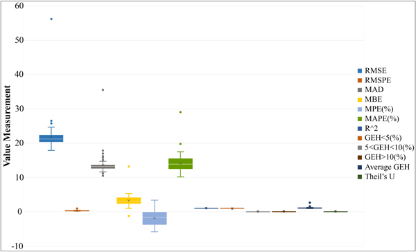
The observed traffic volume (Real Data Sets) and the traffic volume from modelled count data of 99 scenarios were substituted in the formula of each 9 measures listed in Table 1 in order to quantify the model predictive accuracy. From the Box-and-Whisker Plot in Fig. (7), it was found that MPE(%) was the factor with the highest distribution value, followed by MAPE(%) and RMSE. MAD was found to have the highest outliers, as the abnormal values of some scenarios were distant from others in terms of upper extreme and lower extreme positions, which indicated a random sample from a population. However, running dynamic O/D adjustment with a maximum number of iteration of 4 (Scenario 4) could eliminate the outliers of all factor except for MAD. This was because the outliers of MAD were randomly generated, making it hard to clearly summarize the results.
5.3. Statistical Measurement Criteria
The statistical measurement values of the 99 scenarios were compared to the acceptable indicators of each factor in order to determine the statistical measurement criteria. The measurement values that were closest to the acceptable indicators of each factor were set as the upper limit values. Then these upper limit values were used to identify the lower limit values and acceptable ranges. The results suggested that, among all 99 scenarios, there were only 8 scenarios whose measurement values were in the acceptable ranges, as the details shown in Table 3. It was found that the measurement values of Scenario 23 reached the upper limit value of 4 factors: RMSE, MAD, R2, and Theil’s U, and the lower limit value of RMSPE(%). On the other hand, the measurement values of Scenario 25 were found to reach the upper limit value of only one factor, MBE, and reached the lower limit value of 3 factors: MAPE(%), R2, and Average GEH. Moreover, the measurement values of Scenario 43, 47 and 48 were in the acceptable ranges, without reaching any upper or lower limit value. This made the selection of the most accurate scenario for each factor uncertain and difficult to decide. Thus, the multi-factor scoring method was additionally used in the decision-making process.
| Factor | Measurement Values of Statistical Factor |
Acceptable Range |
|||||||
|---|---|---|---|---|---|---|---|---|---|
|
Scenario 23 |
Scenario 25 |
Scenario 31 |
Scenario 42 |
Scenario 43 |
Scenario 47 |
Scenario 48 |
Scenario 49 |
||
| RMSE | 17.87538** | 19.07181 | 19.59906 | 20.80701* | 19.27852 | 19.27595 | 19.64607 | 20.27381 | 2.93163 |
| RMSPE(%) | 0.27900* | 0.26386 | 0.24281 | 0.18500** | 0.20114 | 0.22284 | 0.20225 | 0.23467 | 0.09400 |
| MAD | 10.66007** | 11.68977 | 12.28383* | 12.28053 | 11.67657 | 11.22112 | 11.72607 | 11.97360 | 1.62376 |
| MBE | 1.55116 | 0.97690** | 2.66007 | 2.66997* | 2.02640 | 2.06601 | 2.33333 | 1.90759 | 1.69307 |
| MPE(%) | 0.04017 | 0.20849 | 0.11628 | 0.03044** | 0.06985 | 0.29876 | 0.48677* | 0.40055 | 0.45633 |
| MAPE(%) | 12.43642 | 13.27112* | 12.67264 | 10.52426 | 10.67913 | 10.98155 | 10.16968** | 11.67832 | 3.10144 |
| R2 | 0.99857** | 0.99826* | 0.99837 | 0.99831 | 0.99837 | 0.99843 | 0.99841 | 0.99826 | 0.00031 |
| Average GEH | 0.94410 | 1.04202* | 1.03765 | 0.98174 | 0.96512 | 0.94904 | 0.93759** | 0.99000 | 0.10443 |
| Theil’s U | 0.01648** | 0.01762 | 0.01803 | 0.01911* | 0.01775 | 0.01774 | 0.01807 | 0.01865 | 0.00263 |
* Lower limit value comparing with data set
5.4. O/D Matrix Adjustment Resulting from Applying Multi-Factor Scoring Method
The multi-factor scoring process was conducted by determining the factor score of each 9 measures according to the statistical measurement value and converting it into the conversion value as shown in Equation 10 and Equation 11 in order to avoid bias in calculation and different error ranges.
 |
(10) |
 |
(11) |
Where:
εi = absolute error i,
Aik = acceptable indicators of factor k,
Vmi = measurement value of factor i, and
Coni = conversion value of factor i.
Scoring weight was set based on an assumption that every factor has an equal importance value of 10, indicating that each scenario has a full score of 90. The formula used to calculate the summation of factor scores is given below.
 |
(12) |
Where:
Scoring Weightk = scoring weight of factor k, and
Score = summation of factor score.
According to the calculating results, it was found that the top 5 scenarios that obtained the highest scores were Scenario 23 (80.192), followed by Scenario 43 (79.869), Scenario 42 (79.488), Scenario 25 (78.890), and Scenario 31 (78.554). The measurement values of Scenario 23 reached the upper limit value of 4 factors, which were RMSE, MAD, R2, and Theil’s U, and the lower limit value of RMSP(%). On the other hand, the measurement values of Scenario 43 were in the acceptable measurement range but did not reach any upper or lower limit value. Considering the upper limit value of each factor, it was found that Scenario 25 had a high chance to obtain low scores and ranked last in the list because its measurement values reached the lower limit value of 3 factors: MAPE(%), R2, and Average AGE. However, it turned out that Scenario 25 was ranked in the 4th place. In contrast, Scenario 48 was ranked in the 8th place, although it obtained a score of 77.219 and its measurement values reached the upper limit value of 2 factors: MAPE(%) and Average GEH. Thus, it could be said that the multi-factor scoring method made the selection and ranking process easier to carry out due to its clear and systematic scoring system.
The O/D matrix adjustment of Scenario 23 shown in Table 4 will be used to design a bike route by focusing only on the traffic demand between sub-areas in the municipality or internal sub-area zones (Z), which were the main target of the present research. The resulting O/D matrix adjustment showed that the top 5 sub-areas with the highest traffic demand were Z5 to Z11 (237 PCU/hr), Z9 to Z4 (208 PCU/hr), Z3 to Z16 (175 PCU/hr), Z7 to Z8 (167 PCU/hr), and Z17 to Z2 (133 PCU/hr).
| O/D | Z3 | Z2 | N2 | Z1 | N1 | Z4 | Z5 | Z6 | Z7 | Z8 | Z9 | Z10 | Z11 | Z12 | Z13 | Z14 | Z15 | Z16 | N4 | Z17 | N5 | N3 | Total |
|---|---|---|---|---|---|---|---|---|---|---|---|---|---|---|---|---|---|---|---|---|---|---|---|
| Z3 | 6 | 3 | 1 | 3 | 1 | 2 | 3 | 1 | 14 | 3 | 1 | 2 | 0 | 3 | 3 | 25 | 2 | 175 | 1 | 0 | 1 | 1 | 252 |
| Z2 | 116 | 4 | 1 | 3 | 1 | 2 | 3 | 1 | 60 | 3 | 2 | 1 | 29 | 3 | 3 | 65 | 2 | 4 | 1 | 11 | 1 | 1 | 316 |
| N2 | 8 | 2 | 3 | 82 | 245 | 3 | 3 | 14 | 1 | 39 | 19 | 5 | 3 | 5 | 37 | 0 | 0 | 55 | 5 | 1 | 7 | 102 | 638 |
| Z1 | 29 | 41 | 0 | 3 | 0 | 1 | 2 | 1 | 4 | 2 | 2 | 1 | 3 | 2 | 2 | 1 | 1 | 107 | 0 | 1 | 0 | 0 | 201 |
| N1 | 35 | 5 | 278 | 62 | 6 | 5 | 2 | 14 | 4 | 25 | 3 | 4 | 1 | 4 | 147 | 0 | 2 | 5 | 6 | 11 | 1 | 484 | 1103 |
| Z4 | 0 | 3 | 1 | 3 | 3 | 5 | 1 | 1 | 1 | 9 | 28 | 1 | 86 | 3 | 93 | 65 | 2 | 14 | 1 | 3 | 1 | 1 | 324 |
| Z5 | 26 | 2 | 1 | 2 | 3 | 3 | 6 | 1 | 1 | 0 | 10 | 1 | 237 | 1 | 1 | 0 | 0 | 1 | 1 | 1 | 1 | 1 | 301 |
| Z6 | 0 | 0 | 0 | 0 | 7 | 0 | 0 | 2 | 2 | 1 | 1 | 0 | 70 | 1 | 4 | 1 | 1 | 1 | 0 | 1 | 0 | 0 | 92 |
| Z7 | 15 | 6 | 1 | 3 | 2 | 9 | 85 | 59 | 7 | 167 | 1 | 1 | 143 | 81 | 38 | 27 | 52 | 5 | 1 | 1 | 1 | 1 | 705 |
| Z8 | 3 | 10 | 1 | 1 | 22 | 48 | 1 | 1 | 118 | 4 | 2 | 1 | 2 | 1 | 1 | 14 | 2 | 1 | 1 | 1 | 1 | 1 | 236 |
| Z9 | 0 | 7 | 1 | 93 | 9 | 208 | 33 | 88 | 25 | 1 | 9 | 2 | 56 | 12 | 1 | 1 | 0 | 103 | 1 | 1 | 1 | 1 | 653 |
| Z10 | 1 | 0 | 0 | 0 | 4 | 0 | 0 | 0 | 0 | 0 | 0 | 2 | 92 | 1 | 1 | 1 | 1 | 0 | 0 | 1 | 0 | 0 | 105 |
| Z11 | 1 | 36 | 2 | 121 | 7 | 19 | 34 | 76 | 83 | 1 | 18 | 81 | 11 | 106 | 22 | 132 | 0 | 61 | 1 | 112 | 1 | 1 | 926 |
| Z12 | 1 | 1 | 1 | 4 | 66 | 11 | 96 | 16 | 0 | 0 | 16 | 11 | 1 | 6 | 70 | 3 | 0 | 15 | 1 | 1 | 1 | 1 | 323 |
| Z13 | 1 | 15 | 2 | 20 | 144 | 42 | 32 | 89 | 2 | 0 | 19 | 18 | 1 | 1 | 10 | 1 | 0 | 39 | 1 | 1 | 1 | 0 | 440 |
| Z14 | 0 | 80 | 1 | 1 | 1 | 1 | 34 | 1 | 87 | 24 | 4 | 44 | 78 | 63 | 13 | 5 | 3 | 1 | 1 | 1 | 1 | 1 | 446 |
| Z15 | 54 | 0 | 1 | 0 | 0 | 0 | 1 | 2 | 1 | 17 | 1 | 1 | 1 | 1 | 0 | 38 | 4 | 1 | 1 | 66 | 1 | 1 | 193 |
| Z16 | 3 | 15 | 1 | 18 | 2 | 47 | 15 | 1 | 1 | 1 | 100 | 111 | 59 | 3 | 56 | 1 | 0 | 11 | 1 | 131 | 2 | 0 | 581 |
| N4 | 39 | 3 | 30 | 3 | 7 | 6 | 39 | 2 | 1 | 9 | 2 | 1 | 1 | 1 | 5 | 57 | 95 | 1 | 20 | 1 | 3 | 16 | 341 |
| Z17 | 1 | 133 | 1 | 1 | 1 | 1 | 1 | 0 | 32 | 3 | 14 | 10 | 1 | 0 | 1 | 25 | 1 | 87 | 1 | 4 | 1 | 1 | 320 |
| N5 | 1 | 0 | 1 | 1 | 0 | 1 | 1 | 1 | 2 | 0 | 1 | 0 | 3 | 1 | 0 | 5 | 88 | 61 | 3 | 38 | 3 | 1 | 213 |
| N3 | 58 | 58 | 767 | 22 | 746 | 73 | 2 | 70 | 32 | 57 | 91 | 51 | 4 | 55 | 33 | 60 | 27 | 5 | 64 | 37 | 88 | 17 | 2418 |
| Total | 398 | 423 | 1095 | 447 | 1279 | 487 | 393 | 441 | 475 | 366 | 344 | 349 | 884 | 356 | 542 | 527 | 284 | 753 | 113 | 423 | 117 | 632 | 11129 |
N = external sub-area zone
CONCLUSION
The present research aimed to examine and analyze the estimated traffic demand in Nakhon Sawan Municipality’s road network using AIMSUN simulation model. The model validation method was also used to adjust the origin and destination survey data (O/D matrix) by running dynamic O/D adjustment. The resulting 99 scenarios of O/D matrix adjustment were measured and evaluated with the use of statistical measurement. The goodness-of-fit test was carried out to investigate 9 measures. The multi-factor scoring method was also applied to find the most accurate scenario, representing the estimated traffic demand value. The research results suggested the following conclusions.
- When running dynamic O/D adjustment, the maximum number of iterations should be set to 4 in order to avoid data fluctuation.
- In the process of model validation, after selecting the goodness-of-fit test measures that will be used, it is essential to clearly determine the acceptable values of each goodness-of-fit test measure. This is because the calculating results of each measure are different. The goodness-of-fit test measures can be categorized into 4 groups based on the similarities in results: 1) RMSE, MAD, R2, and Theil’s U, 2) MBE, 3) RMSPE% and MPE%, and 4) MAPE% and Average GEH.
- From Table 3, when using the measurement values to determine the acceptable ranges based on the acceptable indicators of 9 measures, it was found that among all 99 scenarios there were only 8 scenarios that met the criteria. The measurement values of Scenario 31, Scenario 43, Scenario 47, and Scenario 49 did not reach any upper limit value (or the value that was closest to the acceptable indicators), although Scenario 43 had the second highest score, which was considered difficult to predict. Therefore, in the model validation process, the 9 measures were analyzed and evaluated through statistical measurement in order to ensure accuracy and eliminate errors that might occur from using only one goodness-of-fit test measure. The multi-factor scoring method could systematically rank and clearly display the score differences, making it easier for planners and traffic design engineers to make decisions and select appropriate choices.
Based on the research results, it can be summarized that the O/D matrix adjustment of Scenario 23 should be used as the estimated traffic demand between sub-areas in Nakhon Sawan Municipality, according to the traffic engineering principles. This will be helpful for designing bike routes that truly suit the traffic demand, determining urban management policies in terms of construction priority, traffic management measures, promotion of cycling in each area, assessment of economic appropriateness, and investment suitability that are in line with government budgets, and encouraging people to change their daily transportation mode from private cars to bicycles, which consequently leads to energy consumption reduction and sustainable solution to traffic congestion. Future research should build on the findings of this study by further developing traffic simulation models to evaluate the suitability of each bike route design prior to actual construction.
CONSENT FOR PUBLICATION
Not applicable.
CONFLICT OF INTEREST
The authors declare no conflict of interest, financial or otherwise.
ACKNOWLEDGEMENTS
Declared none.

