All published articles of this journal are available on ScienceDirect.

Fast Method to Evaluate Payload Effect on In-Train Forces of Freight Trains
Authors Info & Affiliations
Abstract
Introduction:
This paper introduces a fast method to evaluate the effect of payload distribution on in-train forces.
Methods:
The method is based on Strong Orthogonal Arrays (SOA) and the excellent space-filling properties of Latin Hypercube Design (LHD): SOA-based-LHD is proved to be very efficient in spanning the range of in-train forces for different types of trains (also considering distributed power/braking) and trains operations.
Results:
The distribution of the percentage of braked mass is used to consider the effect of payload distribution on in-train forces. Because of its computational efficiency, the method proposed here can be satisfactorily employed to perform an optimization analysis of train composition.
1. INTRODUCTION
Longitudinal Train Dynamics (LTD), i.e. the relative motion of adjacent railway vehicles running in track direction, has received attention from many researchers in the world. A recent special issue of Vehicle System Dynamics has been devoted to this topic [1] and paper [2] provides an excellent review of this matter. LTD is a key factor in determining the safety of freight train sets: high in-train compressive forces can determine train derailment [3]. High in-train tensile forces are also dangerous, since they can disrupt trains (because of draw gears failure), causing a freight traffic inefficiency. LTD is also important for studying many other topics, such as train energy consumption. LTD simulators are used not only by Research Centres and by Universities around the world but also by Railway Undertakings in order to develop longer and heavier (still safe) freight train sets. A study shows [4] a benchmark of several LTD simulators coming from all over the world.
Among these simulators, only few of them are capable to simulate at the same time air pneumatics and mechanical behaviour of a train. TrainDy, validated against experimental data [5-7], is one of such simulators and it was used in this study to compute LTD of simulated freight train sets. The International Union of Railways (UIC) currently owns TrainDy and it has certified it against more than 30 experimental test campaigns [7]. Beyond TrainDy, in Italy, there are also other LTD simulators claimed to combine the braking system simulation and the computation of in-train forces [8] and [9].
As stated above, one of the applications of LTD simulators is the computation of in-train forces in order to assess the safety against derailment and the risk of train disruption of a freight trainset. One of the simplest ways to achieve this aim is to compare in-train compressive forces (or Longitudinal Compressive Forces -LCF-) against the admissible LCF, measured experimentally following the tests described in reference [10]. In Europe, Railway Undertakings express admissible LCF in terms of 10m LCF (LCF10): 10m LCF is the minimum value (without sign) of LCF occurred in 10m before the current position. The same approach is followed with in-train tensile forces where instantaneous in-train forces are compared against maximum Longitudinal Tension Force (LTF) of draw gears (or draw hooks). Of course, such analyses should consider also fatigue damage, as done e.g. in reference [11].
In-train forces are mainly triggered by train operation (acceleration, braking, and their combinations), train mass and length, braking regime (for pneumatic brake), mass (payload) distribution, braking devices (and their technology), track geometry (uphill, downhill, curves), types of couplers between consecutive vehicles, speed. This paper focuses attention on payload distribution. This topic has been recently addressed in a study [12], where a series of performance indexes has been introduced to study the performance of freight trains in terms of in-train forces (for an extensive parametric study see [13]). The Topic is relevant for Railway Undertakings, especially in Europe, where a series of Codes regulates international freight traffic, such as shown in reference [14], which establishes limits on hauled mass of freight trains. Railway Undertakings know from their operative experience that there can be significant differences in terms of in-train forces depending on freight train set specific arrangement (i.e. permuting vehicle position within train make up). According to a study [14], Railway Undertakings have to statistically simulate freight train sets in order to prove the safety of a new family of trains (e.g. characterized by a new type of braking technology). Moreover, in Europe, there is a new research effort towards longer and heavier trains with distributed power/braking and their assessment requires statistical investigations about the effect of payload distribution on in-train forces.
A study [15] analyses freight trains transporting scrap materials and shows that an optimization of mass distribution in terms of in-train forces is possible by employing a Kriging approach. Of course, such types of trains usually run uniformly loaded and mass optimization is not an issue. On the contrary, for containers’ traffic analysed in this paper, payload distribution optimization results in significant reduction of in-train forces both in compression and in tension.
To this end, in this paper, a particular type of Latin Hypercube Design has been generated based on a new type of Orthogonal Arrays, recently developed in a study [16]. This new approach allows to carry out the payload effect evaluation with a significantly lower number of simulations. With respect to a study [15], this paper also analyses trains with distributed traction/braking, which are currently under investigation in Europe by means of new projects, within the Shift2Rail (S2R) framework [17], to increase freight train efficiency in the near future.
2. METHOD
As already developed by the authors in other works, the literature provides many holistic approaches that can simulate engineering problems. In various fields, there are numerous applications in this direction, among others [18]. For example, one way of gaining this desirable insight into this kind of problems is the use of meta models. They can be used to bridge between various levels of sophistication afforded by varying fidelity physics-based simulation codes, or between predictions and experiments [19]. At this aim, some form of data set relating a series of inputs and outputs is needed typically by sampling the design decision space.
For this reason, when considering evaluation of the payload effect on in-train forces through LTD simulator, a fundamental aspect regards the choice of the trains sample that have to be simulated. The most straightforward approach is to randomly choose trains from a given family of trains and run simulations, adding new train samples as long as statistical parameters (i.e. mean and standard deviation) of in-train force change significantly. Clearly, this kind of approach is not efficient in terms of time and computational resources. For this reason, a crucial feature to address is the underlying experimental design that has to be implemented. In this regard, Space-Filling design could be considered as one of the most suitable designs when dealing with computer experiments, as in the case of freight trains simulations. This is mainly because it allocates the design points, e.g. the sampled trains, as uniformly as possible in order to observe the response in the entire design space, e.g. the in-train forces. The most widely used class of Space Filling design is that of Latin Hypercube Design (LHD) introduced in reference [20]. Various types of LHDs have been developed in the literature. A large class of them are generated using some distance or discrepancy criteria ([21, 22] among others) in order to achieve good space-filling properties. Another important class of LHD is generated through Orthogonal Arrays [23]. Recently, in reference [16], the study developed a new class of Orthogonal Arrays, called Strong Orthogonal Arrays and, in reference [16], the authors have demonstrated the excellent space-filling properties of the LHDs, built from these last types of arrays and called SOA-based-LHD.
Therefore, starting from reference [15] where a LHD based on Sobol sequences with 400 runs was applied, we generated a SOA-based LHD with 64 experimental runs by defining a strategy for representing a train in the design space. As an example, the train is supposed to be divided in 5 sections, representing 5 different destinations of the transported goods: of course, it is not required that all sections have the same number of wagons. Within each section, the payload is freely distributed. Differently from [15], where the percentage of braked mass for each wagon was 100% (ratio between braked mass and wagon mass); in this paper, the object of design space definition is the distribution of percentage of braked mass within each section. In other words, each wagon has its payload and its percentage of braked mass and, because of the proposed method, wagon’s position within the section changes in order to have a desired distribution of percentage of braked mass. In order to describe the geometry of percentage of braked mass distribution with few numbers of variables, it is described as a generalized trapeze by means of two variables as shown in Fig. (1). In this way, the percentage of braked mass, within each section, can have a distribution, which can be: i) uniform, ii) triangular, iii) trapezoidal, according to the values of only two variables. To build each distribution, we denote the length of the train section by B (in terms of number of wagons) and Q demotes the area of each distribution, corresponding to the sum of percentages of braked mass of the wagons. Therefore, every distribution shares the same base (B) and it has the same area (Q). To describe it mathematically, we define two discrete variables, H and X, that could univocally represent the percentage of braked mass distribution for each section. Through the input variable H, it is possible to define the shape of the percentage of braked mass distribution, which can gradually change from the uniform shape to the triangular one: (see Fig. (1)). This figure provides different shapes, according to the different values of variables X and H. For example, for every value of X variable, if H variable is equal to 0, the shape of percentage of braked mass distribution is rectangular (i.e. it is uniform). If H is equal to 1, this shape is triangular, with position of the vertex defined by variable X. For other values of H, the shape is a trapeze, with minor basis becoming smaller for H increasing from 0 to 1. Fig. (1B) shows some of these shapes, emphasizing the fact that all shapes have the same major basis (B) and the same area (Q). In this figure, different style of line type enhances the readability of the figure and has no further meaning.
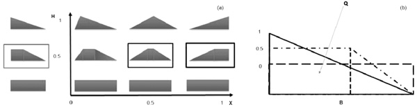
Through the input variable X, it is possible to identify the position of the maximum load along the length of the section: Appendix A provides further details and explicit formulas on how to compute the geometry of the shapes, for every value of X and H, hence not restricted to the combinations shown in Fig. (1A and B).
Therefore, in this example of application of the method, ten factors for SOA-based-LHD are considered: 5 factors related to the shape of the payload distribution H = {H1, H2, H3, H4, H5}, and 5 factors related to the position of the maximum load X = {X1, X2, X3, X4, X5}. The results here obtained for the SOA-based-LHDs represent a further improvement of those obtained in another study [15] through a LHD based on Sobol sequences, as illustrated in paragraph 4. Simulations of this paper employ the following values, for both variables: {0,0.25,0.5,0.75,1}; these values have been selected to regularly cover the geometry of shapes.
3. SIMULATIONS DATA AND ASSUMPTIONS
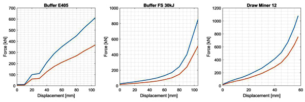
Wagons used for simulations reported in this paper belong to family Rhlmms and Shimmns. Traction unit used is type E405, from Trenitalia. Vehicle data were obtained from Trenitalia database used in reference [24] and are reported in Table (1). Fig. (2) shows the force-displacement characteristics of used couplers; lastly, Table (2) reports the force-speed characteristics of traction unit at maximum level of power.
| Rhlmms | Shimmns | E405 | |
|---|---|---|---|
| Length over buffers [m] | 14.04 | 12.04 | 19.4 |
| Tare [ton] | 20 | 22.5 | 82 |
| Brake pipe diameter [mm] | 32 | ||
| % rotating mass | 4 | 12 | |
| Braked mass Load [ton] | 43 | 58 | 56 |
| Braked mass Empty [ton] | 24 | 26 | - |
| Changing mass [ton] | 40 | 48 | - |
| Buffers | Buffer FS 30kJ | Buffer E405 | |
| Draw gears | Draw Miner 12 | ||
| Brake type | Brake block, cast iron | Disc, constant friction coefficient (0.35) | |
| Brake regime | G (Characteristic timings for brake cylinder filling 24 s and 28 s [7]) | ||
| Speed [km/h] | 0 | 20 | 40 | 50 | 70 | 80 | 90 | 100 | 120 |
| Force [kN] | 560 | 532 | 500 | 490 | 460 | 440 | 424 | 396 | 342 |
| Gradient for power application [kN/s] | 30 | ||||||||
| Gradient for power removal [kN/s] | 16 | ||||||||
This paper analysed two types of train makeups: train_1, having one traction unit in front and 49 wagons for a hauled mass of 2500 ton Table (3); train_2, given by coupling train_1 with train_1b carrying 50 wagons and 2500 ton of hauled mass Table (4). As a result, hauled mass of train_2 is 5000 ton.
The track used for simulations was plane and tangent. Two types of train operations were considered: i) an emergency braking from 30 km/h (label EB); ii) an acceleration from zero increased to 30 km/h, with full power application, followed by an emergency braking applied when 30 km/h speed is reached (label TEB). In case of two connected trains, here it was assumed that emergency braking is applied with a delay of 1s to slave (or second) traction unit in train operation i). In train operation ii), it is assumed that emergency braking (after initial synchronous acceleration) is commanded by the track to the traction unit and it is applied at the same time by traction units. As it is well known, there are many ways to “synchronize” actions between the two traction units. Depending on the actual implementation of communication between traction units and among traction units and track, actual train behaviour can be different from what was modelled here. Anyway, the purpose was to introduce this fast method to reduce the computational time needed to properly simulate the effect of payload distribution on in-train forces. Discussing the architecture of distributed traction/braking trains is out of the scope of this paper.
Trains are divided into sections, each one hauling 500t roughly. More precisely, 49 wagons of train 1 are divided into 5 sections with number of wagons being 9, 11, 9, 9, 11. 50 wagons of train 1b are divided into 5 sections with the following numbers of wagons for each section: 8, 11, 10, 11, 10.
| Wagon | Rhlmms | Rhlmms | Rhlmms | Shimmns | Rhlmms | Rhlmms | Rhlmms | Rhlmms | Rhlmms | Rhlmms |
| Payload | 0 | 34 | 34 | 33.5 | 34 | 35 | 48 | 44 | 35 | 35 |
| # | 1 | 2 | 3 | 4 | 5 | 6 | 7 | 8 | 9 | 10 |
| Wagon | Rhlmms | Shimmns | Rhlmms | Rhlmms | Shimmns | Shimmns | Rhlmms | Shimmns | Rhlmms | Rhlmms |
| Payload | 0 | 32.5 | 34 | 30 | 15.5 | 10.5 | 54 | 0 | 48.5 | 55 |
| # | 11 | 12 | 13 | 14 | 15 | 16 | 17 | 18 | 19 | 20 |
| Wagon | Shimmns | Shimmns | Rhlmms | Rhlmms | Shimmns | Shimmns | Rhlmms | Rhlmms | Rhlmms | Rhlmms |
| Payload | 33.5 | 32.5 | 54 | 35 | 33.5 | 5.5 | 34 | 46 | 34 | 35 |
| # | 21 | 22 | 23 | 24 | 25 | 26 | 27 | 28 | 29 | 30 |
| Wagon | Rhlmms | Shimmns | Rhlmms | Shimmns | Rhlmms | Shimmns | Shimmns | Rhlmms | Shimmns | Rhlmms |
| Payload | 31 | 46.5 | 34 | 3.5 | 30 | 32.5 | 32.5 | 34 | 16.5 | 35 |
| # | 31 | 32 | 33 | 34 | 35 | 36 | 37 | 38 | 39 | 40 |
| Wagon | Rhlmms | Rhlmms | Shimmns | Shimmns | Shimmns | Rhlmms | Rhlmms | Rhlmms | Rhlmms | |
| Payload | 35 | 46 | 0 | 0 | 11.5 | 31 | 34 | 34 | 35 | |
| # | 41 | 42 | 43 | 44 | 45 | 46 | 47 | 48 | 49 |
| Wagon | Rhlmms | Rhlmms | Rhlmms | Rhlmms | Rhlmms | Shimmns | Rhlmms | Shimmns | Rhlmms | Rhlmms |
| Payload | 34 | 35 | 48 | 34 | 34 | 32.5 | 44 | 33.5 | 35 | 16 |
| # | 1 | 2 | 3 | 4 | 5 | 6 | 7 | 8 | 9 | 10 |
| Wagon | Shimmns | Shimmns | Rhlmms | Rhlmms | Shimmns | Rhlmms | Rhlmms | Rhlmms | Rhlmms | Rhlmms |
| Payload | 17.5 | 11.5 | 34 | 34 | 15.5 | 31 | 34 | 35 | 34 | 33 |
| # | 11 | 12 | 13 | 14 | 15 | 16 | 17 | 18 | 19 | 20 |
| Wagon | Rhlmms | Rhlmms | Rhlmms | Rhlmms | Rhlmms | Rhlmms | Shimmns | Rhlmms | Rhlmms | Rhlmms |
| Payload | 30 | 35 | 34 | 34 | 34 | 35 | 10.5 | 0 | 34 | 34 |
| # | 21 | 22 | 23 | 24 | 25 | 26 | 27 | 28 | 29 | 30 |
| Wagon | Rhlmms | Shimmns | Rhlmms | Rhlmms | Shimmns | Rhlmms | Shimmns | Shimmns | Shimmns | Rhlmms |
| Payload | 35 | 33.5 | 34 | 31 | 33.5 | 35 | 15.5 | 13.5 | 16.5 | 34 |
| # | 31 | 32 | 33 | 34 | 35 | 36 | 37 | 38 | 39 | 40 |
| Wagon | Shimmns | Shimmns | Rhlmms | Rhlmms | Rhlmms | Shimmns | Shimmns | Shimmns | Shimmns | Rhlmms |
| Payload | 33.5 | 41.5 | 34 | 15 | 34 | 32.5 | 16.5 | 32.5 | 16.5 | 15 |
| # | 41 | 42 | 43 | 44 | 45 | 46 | 47 | 48 | 49 | 50 |
4. RESULTS
The results are expressed in terms of 10m Longitudinal Compression Forces (LCF10) and instantaneous Longitudinal Tensile Forces (LTF); LCF10 are the minimum (in absolute sense) in-train compression forces applied in 10m before the current position and LTF are the maximum instantaneous in-train tensile forces applied in the current position. Railway Undertakings employ LCF10 to determine safety against derailment caused by high in-train compressive forces and LTF to determine safety against train disruption caused by failure of draw gears.
The results refer to two types of statistical investigations: i) 1000 simulations established by a Monte Carlo (MC) approach where wagons are randomly permutated within each section; ii) 64 simulations established by SOA-based-LHD described in paragraph 2. These two types of statistical investigations were repeated for the two train operations described at the end of paragraph 3. 1000 simulations were of the same order of magnitude of the simulations performed by Railway Undertakings for similar types of investigations. This is a good trade off among accuracy and efficiency in this type of study. In UIC CODE 421 [14], it is required to compute mean and standard deviation of data and to consider a number of statistical runs able to catch their significant variation, and this has been done in order to internally check the accuracy of the results.
Fig. (3) shows the flowchart of model implementation from input data to simulations results.
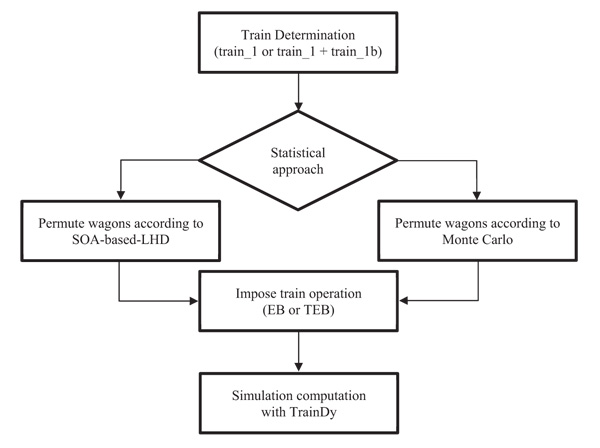
Fig. (4) reports cumulative functions referred to LCF10 and LTF: circles refer to SOA-based-LHD and stars to Monte Carlo. In Fig. (4), (a) and (b) refer to an emergency braking performed by train 1; (c) and (d) refer to an emergency braking performed by connection of train_1 and train_1b (i.e. connected train); (e) and (f) refer to an acceleration followed by an emergency braking performed by a connected train.
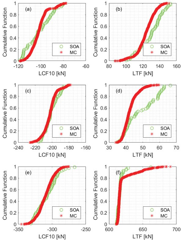
Curves shown in Fig. (4) are generally similar and for single train (a) and (b)– provide similar values for minimum LCF10 and maximum LTF (this result has been found also in [15]). For connected train – from (c) to (f)– there are some differences in terms of minimum LCF10 and maximum LTF. Table (5) provides a synthesis of such values, which are important from the safety point of view (on the contrary, maximum LCF10 and minimum LTF are important for payload optimization).
| – | EB, train_1 | EB, train_2 | TEB, train_2 | ||||
|---|---|---|---|---|---|---|---|
| – | min | max | min | max | min | max | |
| LCF10 | -119,1 | -79,8 | -215,7 | -181,4 | -331,7 | -266,6 | SOA |
| -118,8 | -77,4 | -226,3 | -177,9 | -345,5 | -275,4 | MC | |
| LTF | 100,3 | 152,9 | 35,0 | 66,4 | 611,4 | 662,1 | SOA |
| 87,1 | 151,1 | 33,8 | 59,7 | 610,4 | 691,0 | MC | |
Even if differences in terms of maximum and minimum values are important, it is even more important comparing the two statistical investigations by means of statistical indexes [25]. To this end, Table (6) compares the results in terms of mean and standard deviation; it quantitatively shows the coherence of the two statistical investigations, even with different levels of approximation for different cases.
| – | EB, train_1 | EB, train_2 | TEB, train_2 | ||||
|---|---|---|---|---|---|---|---|
| – | µ | σ | µ | σ | µ | σ | |
| LCF10 | -101,4 | 11,1 | -200,9 | 8,2 | -307,5 | 15,1 | SOA |
| -101,6 | 7,7 | -202,6 | 8,2 | -309,6 | 12,1 | MC | |
| LTF | 129,4 | 14,0 | 48,5 | 9,1 | 616,6 | 6,7 | SOA |
| 123,8 | 10,8 | 42,5 | 4,2 | 620,9 | 14,0 | MC | |
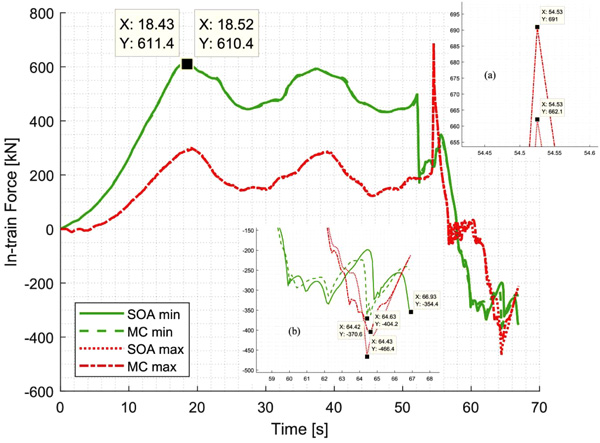
To make the analysis more short and interesting, the focus was only on train operation TEB, performed on connected trains. The behaviour shown in Fig. (4) (f) is typical for this train operation. For this train operation, during the first acceleration phase (almost independently from payload) usually maximum LTF are observed; anyway, during the first phases of emergency braking application, maximum of LTF can occur, for several payload distributions. The latter behaviour is also affected by gradient of power reduction and application at traction unit. As already mentioned, because of emergency braking (supposed commanded by the railway), the power is removed instantaneously in these simulations; if power would have been removed slowly, dynamic oscillation would not have occurred. Fig. (5) shows the time evolution of instantaneous in-train forces for minimum and maximum values of Fig. (4) (f). The results of two statistical investigations were observed to be very similar. In Fig. (5), labels “min” and max” mean that it shows the time evolution of the simulations with, correspondingly, lower maximum (611.4kN and 610.4kN for SOA and MC, respectively) LTF and with higher maximum (662.1kN and 691kN for SOA and MC, respectively) LTF in Fig. (4) (f). This figure has two zoomed areas, showing the time evolution in the nearby of maximum (a) and minimum (b) instantaneous in-train forces. Only by zooming the figure, it is possible to see the differences between the reported time evolutions, emphasizing the fact that the results they provide, are generally very similar except in some local areas. Peaks' quantification is given in Fig. (5A and 5B) for LTF and LCF, respectively. It is similar to the data shown in Table (5) for LTF, but is different for LCF, since Table (5) reports LCF10; whereas Fig. (5) refers to the instantaneous in-train Compressive Forces (LCF).
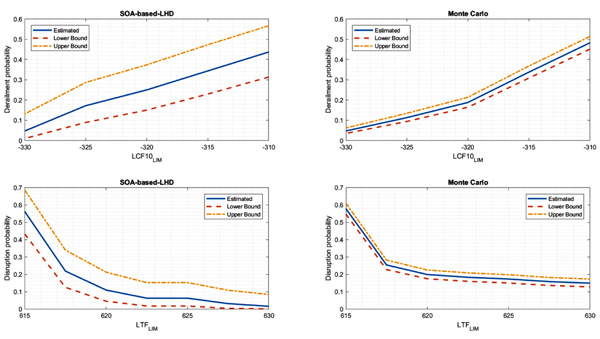
Fig. (6) reports the estimated probability of train derailment and disruption according to the supposed limits in terms of LCF10 and LTF. The type of wagon and its payload determine the limits in terms of in-train compressive forces; reference [14] provides a way to compute it. In this reference, a method to compute estimated probability and its boundaries according to Clopper-Pearson interval has also been described. The type of draw gear and its fatigue life provide limits in terms of in-train tensile forces. The results shown in Fig. (6) show that estimated probabilities and its boundaries are coherent between the two statistical investigations: of course, SOA-based-LHD provides bigger interval respect to Monte Carlo because of its lower number of simulations.
Differences in terms of results should be evaluated in light of the increase of computational efficiency (more than one order of magnitude) brought by SOA-based-LHD sampling.
4.1. Implications and Discussion
Freight trains in Europe are usually equipped with one or two traction units placed at the beginning of the train. There are some cases of distributed power and braking where the traction units are placed at the beginning and at the end of the train and there are drivers in both the traction units. As mentioned in the Introduction, there is a research activity in this field, financed by European Commission in the framework of Shift2Rail project [17], aiming to set the operation distributed power and braking trains with driver(s) only in the master traction unit. Because of its international certification, TrainDy software is one of the tools entrusted for the computation of Longitudinal Train Dynamics for such trains, by European Railway Undertakings. For new train sets’ assessment, it is necessary to statistically compute trains with random displacement of wagons. The results were computed with TrainDy, referring to a challenging situation of containers traffic where each train is divided into 5 sections. In case of mass optimization of this type of trains, a random permutation of wagons’ position is performed. The aim of these studies was to compute the probability of overcoming certain levels of LCF10 or LTF. This problem is important because it is related to train derailment (for LCF10) and to train disruption (for LTF). The Proposed method allows the computation of such probabilities with a reduced computational effort, as the achieved results demonstrate.
CONCLUSIONS
Train characterization in terms of length, hauled mass, type of wagons and their connections is not enough to assess the amount of in-train forces. The experiences of Railway Undertakings and of researchers in the field of Longitudinal Train Dynamics show that it is important to consider train operations and payload distribution. This paper considered the type of train and train operation as a parameter and performs a series of statistical investigations on payload distribution. Actually, the percentage of braked mass is the parameter under investigation in statistical computations. Two types of statistical investigations are performed: 1000 simulations established on a pure Monte Carlo approach and 64 simulations established were SOA-based-LHD described in paragraph 2. Through a significantly lower number of experimental runs, satisfactory results in terms of optimization of the payload distribution have been achieved. The results also consider connected trains, which are thought to be the future of heavy haul freight transportation in Europe. This shows that with the proposed method, it is possible to study the most dangerous payload distributions and optimized payload distributions, with a relatively small computational effort. Further studies will be carried out in order to assess the number of train sections that can be handled by means of the proposed model.
SHORT NOTES ON PAYLOAD ARRANGEMENT
As paragraph 2 describes, during the optimization of payload distribution each section keeps the overall transported payload and the number of wagons; this, in turn, is as to say that they keep the same percentage of braked mass and number of wagons. According to symbols used there, this is to say that area Q and base b remain the same. Each sample of design of experiment is identified by particular values of parameters H and X, which refer to specific train section. In order to avoid too similar distributions of percentage of brakes mass (λ), parameters H and X (bounded in interval 0-1) change with a step of 0.25. According to H value, λ distributions can have following shapes:
• H=0, rectangle
• H=0.25;0.5;0.75, trapeze
• H=1, triangle
Parameter X represents the “position” where λ starts to decrease. All above shapes can be described by a trapeze (even degenerate). In order to provide simple formulas for describing shapes of λ distribution in terms of (H, X) couples, it is useful to refer to Fig. (A1).
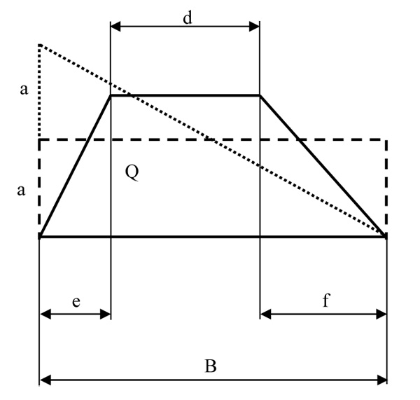
Since all λ distributions share the same area Q, which represent the sum of percentages of braked mass of wagons that belong to specific sub-section and the number of wagons (B), it is possible to define the quantity a =  , as the height of the rectangle, when H parameter is equal to 0. Of course, if H=1, the height of the triangle is c = 2a .
If λ distribution is trapezoid: Equation Chapter (Next) Section 11
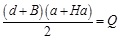 |
(A1.1) |
By which:
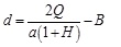 |
(A1.2) |
In order to define other quantities, it is possible to assume:
• e = 0, if X = 0; e = B-d, if X = 1
• f = B-d, if X = 0; f = 0, if X = 1
Since, d + e + f = B,it results, in general:
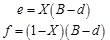 |
(A1.3) |
Above formulas allow description of λ distribution for each couple (H, X).
Of course, since each wagon has an assigned percentage of braked mass, actual λ distributions differ from the target ones, hence wagons have to be disposed in a way to reduce the error with respect to target distribution.
CONSENT FOR PUBLICATION
Not applicable.
CONFLICT OF INTEREST
The authors confirm that the article content has no conflict of interest.
ACKNOWLEDGEMENTS
Declared none.

