All published articles of this journal are available on ScienceDirect.

Bus Passenger Demand Modelling Using Time-Series TechniquesBig Data Analytics
Abstract
Background:
Public transport demand forecasting is the fundamental process of transport planning activity. It plays a pivotal role in the decision making, policy formulations and urban transport planning procedures. In this paper, public bus passenger demand forecasting model is developed using a novel approach. The empirical passenger demand for a bus depot is modelled and forecasted using a data-driven method. The big data generated by Electronic Ticketing Machines (ETM) used for issuing tickets and collecting fares is sourced as the data for demand modelling. This big data is time indexed and hence has the potential for use in time-series applications which were not previously explored.
Objectives:
This paper studies the application of time-series method for forecasting public bus passenger demand using ETM based time-series data. The time-series approach used is the four Holt-Winters’ modeling methods. Holt-Winters’ additive and multiplicative models with and without damping have been empirically compared in this study using the data from the inter-zonal buses. The data used in the study is a part of the transaction on ticket sales by Kerala State Road Transport Corporation (KSRTC) maintained at the Trivandrum City depot of an Indian state Kerala, for the period between 2010 and 2013. The forecasting performance of four time-series models is compared using Mean Absolute Percentage Error (MAPE) and the model goodness of fit is determined using information criteria.
Conclusion:
The forecasts indicate that multiplicative models with and without damping, which better account for seasonal variations, outperform the additive models.
1. INTRODUCTION
The increasing urban population plays a pivotal role in the growing travel demand, which in turn causes the transport crisis in Indian cities. The congested roads, slow-moving traffic, lack of road space and increased travel time are few issues faced by urban travellers. In addition to this, the lack of reliable public transport fuels the transport crisis. An attractive and safe public transport system helps in shifting the travel mode from private to the public mode of travel. Therefore, to meet the growing travel demand, with the existing infrastructure and a minimum number of vehicles, it is required to improve the public transport system. In India, very few cities have planned, regulated and monitored public transport operation. It is mainly due to the lack of huge database required for the estimation of passenger demand. Also, there is a need for frequent updating and analysis of the demand scenario on a periodical basis for the planning of public transport. The data needed for transportation planning is conventionally collected using manual methods or field-based observations. It includes bus occupancy survey, boarding-alighting surveys and passenger interviews. These field data collection techniques are time-consuming and require a lot of human resources. The data collection also incurs a substantial financial burden on the already distressed public transport agencies.
Another method of data collection is automated or technology-based methods. The technology-based methods include Automatic Passenger Count (APC) system [1], Automatic Fare Collection (AFC) system [2] and Automatic Vehicle Location (AVL) system [3]. These Automatic Data Collection (ADC) systems [1, 4-6] used for daily operations have generated an enormous database that can be used for various applications in the transport industry. The data collected from diverse sources of ADCs have distinct features and varied applicability. For example, AVL device is installed on a bus to track the location of the bus. On the other hand, APC gives the number of passengers by receiving “On or Off counts” or sometimes “On and Off counts” using sensors installed near the doors. In some cases, APC data is the by-product of fare transactions as the data is recorded when the passenger pays for the ticket [4]. When a passenger purchases a ticket, AFC data gets recorded. The AFC data gives the details regarding the origin, destination, number of passengers, fare and ticket type. However, in the proof-of-payment type AFC systems, the possibilities of fare evasion exist and thus the passenger demand is underestimated. Hence, there is a need to establish a procedure to tackle the fare evaders to ensure that the demand data of all the passengers [7].
In India, the emergence of electronic fare collection system has become the fundamental system of automated data collection in the public transport industry. In the last decade, most of the transport operators have installed Electronic Ticketing Machines (ETM) for issuing tickets and for fare collection. In the case of a developing country like India where smart card or travel card facilities are not commonly available, it is required to develop methods to use the readily available alternative data sources like ETMs. The ETMs generate a large amount of data, known as big data, pertaining to the number of passengers, time of ticket issuing, fare collected, earnings per kilometre and operated kilometre [4]. The ETM data is available on a time scale since the time of ETM implementation for the entire public transport network and the fleet. This readily available data can be used for passenger demand estimation, performance evaluation and for developing strategic plans. The transit agencies use this ETM data for improving the operating profit and performance evaluation. However, the potential of ETM data for passenger demand estimation is not explored in the literature. Therefore, this study tries to analyse the time-series ETM data for passenger demand modelling and forecasting for a depot.
2. LITERATURE REVIEW
Time-series is a chronological observation of any variable over time [8]. Time-series approach involves the collection of historical data, data pre-processing, data mining using the right data mining tools and understanding the underlying characteristics of the time-series data [9]. Then the patterns in the data are used to build a model which can be used for forecasting the future observations. Time-series modelling methods include exponential smoothing techniques, family of Autoregressive (AR) models, Autoregressive Conditional Heteroscedasticity (ARCH) models and soft computing techniques.
Exponential Smoothing Techniques are simple tools used for smoothening the time-series data and subsequently forecasted to get future observations. The time-series data is smoothened using a smoothening parameter by eliminating the noise in the data to get the pattern in the series. The weighted averages of the past observations are used for forecasting [10]. When new data points are available, the weights of the older data points decay exponentially. The newer the data the higher is the weight, and the older the data the lower the weight. The weights assigned to the observations are determined by the smoothing parameters. Exponential smoothing techniques consist of different variants like Simple Exponential Smoothing (SES), Double Exponential Smoothing (DES) and Holt-Winters’ method. These variants of exponential smoothing are intended for different scenarios.
Simple exponential smoothing can be used when the data has no significant trend and seasonality. In double exponential smoothing, a trend variable is incorporated to account for the slope or trend in the time-series data. The SES has a single smoothening equation for level while the DES has two smoothening equations for level and trend. When the data has both trend and seasonality, seasonal Holt-Winters’ model is used. Holt-Winters’ model has three smoothening equation for level, trend and seasonality. Holt-Winters’ model has two variantsadditive model and multiplicative model. The additive model is used when the seasonality is almost constant throughout while the multiplicative model is used when the seasonality changes proportionally to the level of the series.
Holt-Winters’ models are used in the various forecasting problems such as air transport demand [11, 12], electricity demand [13], automobile petrol demand [14], agricultural commodities [8], and modelling of traffic flow [6]. Li et al. considered various forecasting techniques like linear trend model, exponential trend model, quadratic trend model, Holt’s linear model, Holt-Winters’ model, partial adjustment model and Autoregressive Integrated Moving Average (ARIMA) model to evaluate the automobile fuel demand forecasting performance empirically. It has been identified that for both seasonal and non-seasonal data, quadratic trend model gave optimum forecasts. Ghosh et al. [15] used three different time series models, viz. random walk model, Holt-Winters’ exponential smoothing technique and seasonal ARIMA model for modelling traffic flow in Dublin. The data used for the study was obtained from loop detectors in the city centre of Dublin. It was found that data had a strong daily seasonal pattern and a stable trend. The forecasts of seasonal ARIMA and Holt-Winters Model were highly competitive with Holt-Winters method having slightly better forecasts. Brandt and Bessler [16] compared the performance of seven forecasting models by examining their performance over 24 quarter. The methods include various exponential smoothing methods, ARIMA model, expert judgement, econometric model and simple average models. The performance of the models was evaluated using the Mean Absolute Percentage Error (MAPE) and Mean Square Error (MSE). The data having a quarterly seasonality was forecasted accurately by the ARIMA models. Taylor [13] studied the electricity demand forecasting using data having double seasonality. The electricity demand data recorded at half-hourly intervals contains both intra-day and daily seasonality. To capture the double seasonality in the data, a double seasonal Holt-Winters’ method was used. It was found that the double seasonal method outperformed the traditional Holt-Winters’ method.
To summarize the literature reviewed, it can be stated that exponential smoothing methods are used for various forecasting applications. Each of the exponential smoothing methods has its own advantages over the other like simple exponential smoothing being used when the data has no trend and no seasonality. Data having seasonality and trend must be modelled using double exponential smoothing. Holt-Winters’ method is used for data with both seasonality and trend. While the data having multiple seasonality have to be forecasted using double seasonal Holt-Winters’ method.
Despite the accumulating evidence of the ability of the exponential smoothing techniques for demand forecasting, there is limited literature that focuses on the application of the exponential smoothing method for bus passenger demand forecasting. Therefore, this paper presents an empirical study on modelling and forecasting daily bus passenger demand using the four Holt-Winters’ time series method. The research question addressed in this paper is: what is the forecasting performance of various Holt-Winters’ modelling methods in the context of ETM based time-series public bus transport data. To address this issue, we measure the forecasting error using Mean Absolute Percentage Error (MAPE) and model goodness using information criteria values. The MAPE value of less than 10% is acceptable in the case of most ITS applications [17].
3. HOLT-WINTERS’ EXPONENTIAL SMOOTHING METHODS
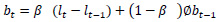
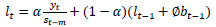
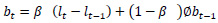
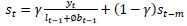
Holt-Winters’ forecasting model consists of four equationsone forecast equation ( ) and three smoothening equations, one each for level (lt), trend (bt) and seasonality (st). These four equations are the component form representation of Holt-Winters’ exponential smoothing model. Holt-Winters’ additive model and multiplicative model with and without damping are explained in the following subsections.
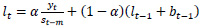
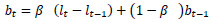
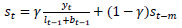
3.1. Holt-Winters’ Additive Method
The formulation of Holt-Winters’ additive model is given below.
 |
(1) |
 |
(2) |
 |
(3) |
 |
(4) |
Where,
is the forecast equation. It is the estimate of yt+h based on the data y1, y2, …, yt
lt is the level (or smoothened value) of series at time t,
bt is the estimate of trend or slope of the series at time t,
st is the seasonal estimate of the time series at time t,
α is the smoothening parameter for level,
β is the smoothening parameter for trend,
γ is the smoothening parameter for seasonality,
h is the forecast horizon
m is the seasonality in the data
k is the integer part of (h-1)/m conforming that the seasonal indices come from the latest observations.
3.2. Holt-Winters’ Multiplicative Method
The components of Holt-Winters’ Multiplicative Model, having the parameters as explained above, is given in the following equations.
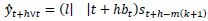 |
(5) |
 |
(6) |
 |
(7) |
 |
(8) |


4. STUDY AREA
Thiruvananthapuram, also known as Trivandrum is selected as the study area. The Trivandrum city is the capital of Kerala state, which is in the southernmost part of India. Thiruvananthapuram district is situated between north latitudes 80 17’ and 80 54’ and east longitudes 760 41’ and 770 17’. The city comprises of thickly populated low land and is the most populous and largest city in Kerala with an area of 214.86 sq. km. The city has a population of 1032292 as per census 2011 making it the most populous city in Kerala with an average population density of 4454 persons’/sq. km [18]. The city bus is the most important mode of public transport in the city. In Thiruvananthapuram city, public transport is dominated by state-owned Kerala State Road Transport Corporation (KSRTC) buses. This study uses the passenger data of the inter-zonal buses of Trivandrum Depot. The ticketing details of all the buses and routes were collected from the depot for the period between 2011 and 2013. The map of Trivandrum city along with the wards is given in Fig. (1).
5. DATA COLLECTION AND ANALYSIS
The data used in the study is a part of fare transactions of issuing tickets in buses of Trivandrum City Depot using the Electronic Ticketing Machines. The ticket includes details of the number of passengers, fare, ticket type, route, origin, destination and the time of ticket issued.
5.1. Data Source-The Electronic Ticketing Machines
Electronic Ticket Machine (ETM) is a handheld device used by the ticket collector for issuing the tickets to the passengers using the bus. The e-ticket contains details of the bus, information of the route and trip details. The machine records information such as the bus type, bus number, minimum fare, fare increment, fare stages, bus stop details, route number, passenger type and the number of passengers [4]. The raw data from the ETM has to be processed to obtain the required passenger demand data.
The advantages of using ETM data source over other surveys are listed below [2, 4, 19]:
- Reduced time and cost requirement
- Large sample size
- No bias in data collection
- Frequent data collection and estimation
- Data analysis can be done for any time period
The challenges of using ETM data source are as follows:
5.2. Time Series Analysis
The data used were daily time-series data from 01-01-2012 to 09-10-2013. Fig. (2) shows the time-series plot for the observed data which is the number of passengers plotted against time in days. It can be observed that the data has a decreasing trend and outliers.
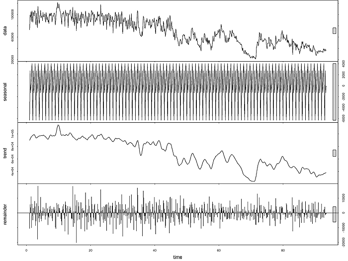
The data is further decomposed into various components like trend, seasonal and irregular as shown in Fig. (3). It can be observed that there exists a seasonality of seven. This seasonality can be further used in the Holt-Winters’ modelling.
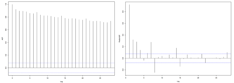
The Autocorrelation Function (ACF) and Partial Autocorrelation Function (PACF) of the observed data is plotted in Fig. (4) to identify the correlations of the data with its lagged values. ACF shows significant correlations between the lagged values and the presence of seasonality in the data. The slow decrease in the ACF denotes the presence of a trend in the data, and hence it is non-stationary. The scalloped shape in the ACF is due to the influence of seasonality in the data. The PACF plot confirms the presence of seasonality of seven.


| α | β | γ | ϕ | σ | AIC | AICc | BIC | MAPE | |
|---|---|---|---|---|---|---|---|---|---|
| Holt-Winters’ Additive Method | 0.472 | 0.0025 | 0.084 | - | 7387.43 | 14994.18 | 14994.70 | 15047.30 | 8.57 |
| Holt-Winters’ Multiplicative Method | 0.458 | 0.0028 | 0.060 | - | 0.1141 | 15048.62 | 15049.14 | 15101.74 | 8.30 |
| Holt-Winters’ Damped Additive Method | 0.465 | 1e-04 | 0.083 | 0.867 | 7360.59 | 14990.67 | 14991.27 | 15048.21 | 8.55 |
| Holt-Winters’ Damped Multiplicative Method | 0.492 | 1e-04 | 0.016 | 0.975 | 0.1131 | 15038.51 | 15039.12 | 15096.06 | 8.29 |
6. EMPIRICAL COMPARISON OF THE RESULTS AND DISCUSSION
The empirical comparison of the results of the methods is made by measuring the forecast accuracy of the models. The data from 01-01-2012 to 09-09-2013 was used for model calibration and parameter estimation while the last 30 days’ data was used for model validation.
The parameters of the model are estimated by maximizing the likelihood value using MLE (Maximum Likelihood Estimation) method. The probability of the data arising from the model is known as the likelihood. For a good model, the likelihood value will be more significant. In the case of the additive model, maximizing the likelihood gives the same result as minimizing the sum of squares. But it is not the same for multiplicative models. The estimated parameters are presented in Table 1.
The smoothening parameters are α ,β and γ while ϕ is the dampening parameter. The parameter α governs the amount of change in the successive levels; the high value of α leads to rapid changes in the levels while a low value of α leads to a smooth change in the levels. In the damped method, the smoothing parameter β is having a small value indicating that the slope or trend component change very little over time. Similarly, a small value of γ indicates that the seasonal component also changes slowly over time.
The minimum of Akaike Information Criteria (AIC), Corrected AIC (AICc) and Bayesian Information Criterion (BIC) values are used to identify the best model along with Mean Absolute Percentage Error (MAPE). Comparing the AIC, AICc and BIC value of all the four models, it can be observed that Holt-Winters’ Damped Additive method have minimum value followed by Holt-Winters’ Damped Multiplicative model. But, it can be noted that the standard deviation (σ) of the additive model is very high compared to the multiplicative model. Since, both these models have the same number of parameters to be estimated, we can compare the MAPE of the models. The Holt-Winters’ Damped Multiplicative model has the least MAPE of 8.29 among all the models. Therefore, it is selected as the best model. To conclude, it can be stated that for a time-series data with seasonality, the Holt-Winters’ Damped Multiplicative method provides accurate and reliable results.
CONCLUSION
The development of big data concept and analytics has contributed enormously in transport planning and operations. The ETM’s, being one of the big data sources in public transport operations, has generated an enormous database including the number of passengers using the bus, operated kilometres, revenue collected and other trip details. This big data is timeindexed and hence has the potential for use in time-series applications which were not previously explored in the literature. Therefore, this paper studied the application of time-series method for forecasting public bus passenger demand using ETM based time-series data. Holt-Winters’ additive and multiplicative models with and without damping have been empirically examined in this study using the ETM data from the inter-zonal buses of Trivandrum City depot. The forecast performance of the four Holt-Winters’ models is compared using MAPE. The following are the primary conclusion from this study:
- The analysis of bus passenger demand data reveals that daily seasonality is present in the data. The seasonality of seven is indicative that one week lagged data show a significant correlation with the original time-series observations.
- Holt-Winters’ multiplicative models with and without damping outperform the additive models. However, the MAPE of all the models is less than 10% with the damped multiplicative model having the least value of 8.29.
- The standard deviations of the multiplicative models are negligible suggesting that the model fit is good. Therefore, Holt-Winters’ Damped Multiplicative method provides better forecasts in the case of seasonal data.
FUTURE WORKS
In the future, further research should be undertaken to determine whether there exists multiple seasonality in the data. Then, the multiple seasonality must be addressed using either seasonal ARIMA or double seasonal Holt-Winters’ method.
LIST OF ABBREVIATIONS
| ETM | Electronic Ticketing Machines |
| KSRTC | Kerala State Road Transport Corporation |
| MAPE | Mean Absolute Percentage Error |
| APC | Automatic Passenger Counts |
| AFC | Automatic Fare Collection |
| AVL | Automatic Vehicle Location |
| ADC | Automatic Data Collection |
| AR | Autoregressive |
| ARCH | Autoregressive Conditional Heteroscedasticity |
| SES | Simple Exponential Smoothing |
| DES | Double Exponential Smoothing |
| ARIMA | Autoregressive Integrated Moving Average |
| MSE | Mean Square Error |
| ACF | Autocorrelation Function |
| PACF | Partial Autocorrelation Function |
| AIC | Akaike Information Criteria |
| MLE | Maximum Likelihood Estimation |
| BIC | Bayesian Information Criterion |
AVAILABILITY OF DATA AND MATERIALS
The data used for this study is a part of fare transactions in issuing the tickets in the buses of Kerala State Road Transport Corporation using Electronic Ticketing Machine. The data sets used and/or analyzed during the current study are available from the corresponding author.
FUNDING
None.
CONSENT FOR PUBLICATION
Not Applicable
CONFLICT OF INTEREST
On behalf of all authors, the corresponding author states that there is no conflict of interest.
ACKNOWLEDGEMENTS
Declared none.

