All published articles of this journal are available on ScienceDirect.
Data Processing Techniques for Real-Time Traveler Information: Use of Dedicated Short-Range Communications Probes on Suburban Arterial
Abstract
Background:
As wireless communication technologies evolve, probe-based travel-time collection systems are becoming popular around the globe. However, two problems generally arise in probe-based systems: one is the outlier and the other is time lag. To resolve the problems, methods for outlier removal and travel-time prediction need to be applied.
Methods:
In this study, data processing methods for addressing the two issues are proposed. After investigating the characteristic of the travel times on the test section, the modified z-score was suggested for censoring outliers contained in probe travel times. To mitigate the time-lag phenomenon, a recurrent neural network, a class of deep learning where temporal sequence data are normally treated, was applied to predict travel times.
Results:
As a result of evaluation with ground-truth data obtained through test-car runs, the proposed methods showed enhanced performances with prediction errors lower than 13% on average compared to current practices.
Conclusion:
The suggested methods can make drivers to better arrange their trip schedules with real-time travel-time information with improved accuracy.
1. INTRODUCTION
Real-time travel-time information is an essential element of modern traffic management systems. It enables drivers to make detours in their routes to less congested ones or to adjust their trip schedules to avoid traffic jams. With the development of wireless communication technologies coupled with the increased market penetration of relevant on-board units, probe-based travel-time systems are being deployed worldwide due to their ability to directly obtain link travel times. In Korea, freeways and major arterials are equipped with Dedicated Short-Range Communications (DSRC) scanners (Fig. 1). DSRC is originally used for the electronic toll collection systems in Korea and around 80% of vehicles are equipped with DSRC on-board units, indicating that probe sample size is not a critical issue.
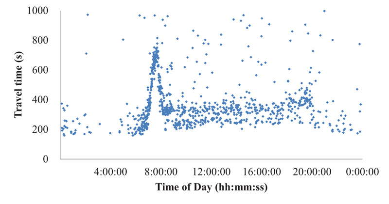
However, the DSRC systems installed on suburban arterials on which many intersections and roadside stores exist inevitably generate substantial outliers due to intermediate stops at stores and/or gas stations, exit/entry maneuvers on the route, U-turns, driving illegally on the shoulder lane during congestion, and so on. Moreover, DSRC scanners cannot identify the direction of a detected probe, so if a probe makes a round trip on the roadway section, the probe is detected twice by the scanner. In this case, the second detection generates an abnormally long travel time and should be classified as an outlier. The severity of the outlier problem of the study site is exemplified in Fig. (2), where substantial outliers are observed. If these outliers are not properly treated, the travel-time information could be useless.
Another issue to be addressed is a time-lag phenomenon. Probe travel times obtained using DSRC scanners inevitably include time lags equivalent to the travel times experienced by the probes on the segment because they, which normally called arrival time-based travel times, are to be computed after probes complete the trip. However, the drivers who receive the arrival time-based travel-time information experience the departure time-based travel time (Fig. 3). Therefore, applying a prediction technique is more emphasized in probe-based real-time systems than conventional detector-based systems.


To resolve the above-mentioned problems, data processing methods for outlier removal and travel-time prediction were proposed in this study. After identifying the problems in the current practices, new methods were developed to resolve the problems. Investigation on the distribution of the probe travel times revealed that the current outlier removal technique based on the z-score is inappropriate for the test section. Therefore, an alternative method is suggested that takes the travel-time characteristic into account. Also, a widely recognized deep learning model is employed to enhance the travel-time prediction performance. The details will be described in the subsequent chapters.
2. LITERATURE REVIEW
Studies have been performed to deal with outlier problems in probe-based travel-time systems. The Southwest Research Institute [1] developed the TransGuide algorithm, which uses a simple validity window calculated from the observations in the previous aggregation interval. Clark et al. [2] suggested a statistical technique to filter outliers contained in probe travel times collected using devices that recognize vehicle registration numbers. Dion and Rakha [3] suggested an algorithm to estimate travel times with an assumption that they follow a lognormal distribution. Ma and Koutsopoulos [4] proposed a median filter that uses the median, instead of the mean, as a measure of location. Boxel et al. [5] developed a method that filters out outlying observations using a confidence interval predefined through Greenshield’s traffic flow theory. Soroush and Bruce [6] invented an adaptive outlier detection algorithm that uses historical and current interval data gathered on signalized arterials to determine a validity window. Park and Kim [7] proposed a model to filter outliers in travel time data obtained using DSRC on the interrupted traffic flow section.
Several methods for predicting real-life travel times have been adopted for the past several decades. Among the most reputed methods are the Kalman Filter (KF), Artificial Neural Network (ANN), Time Series Analysis (TSA), and the k-Nearest Neighbor (k-NN) technique. KF, firstly proposed by R. E. Kalman [8], is an algorithm that utilizes observations in a time sequence and generates estimates of unknown variables [9]. ANN, created with inspiration from the biological neural networks, is a computing algorithm that learns from archived historical measurements to conduct a certain mission [10, 11]. Among various ANN algorithms, recurrent neural network algorithms that mostly treats with measurements in a time sequence are recently receiving much attention from developers on the globe [12-14]. TSA is a method for analyzing time-series data to forecast unknown variables based on the values observed earlier [15, 16]. k-NN, a sort of nonparametric technique mostly adopted for classification or regression, has widely exploited to forecast real-time travel times [17-26]. In k-NN methods, the input variables are the k closest training instances in the feature domain.
3. TEST SITE DESCRIPTION
Probe travel times collected from DSRC scanners installed on a signalized arterial in Pyeong Taek region, South Korea (Fig. 4) were used for evaluating the data processing techniques proposed in this study. Traffic on the 4 km stretch of the highway with two lanes in each direction is controlled by six traffic signals. Due to intermediate stops by the signals, the average travel speed on the section under low volume situations is around 50 km/h even though drivers can drive up to 80 km/h by the regulation.
Individual probe travel times, as shown in Fig. (5), without outlying observations, exhibited a normal commuter corridor with apparent morning peak hours from 7:00 to 9:00 a.m. during weekdays. Travel times during peak hours are 3-4 times higher than the remaining hours, indicating that real-time traveler information is highly stressed during peak hours.
4. OUTLIER TREATMENT
4.1. Current Practice for Outlier Removal
Presently, an outlier removal technique based on the z-score is employed that uses the z-score of observations to censor outlying observations (refer to equations 1-3). Previous 30 probe samples, which is the minimum sample size for the application of the Gaussian distribution are used to compute the relevant statistics. However, the technique has been intuitively applied to the system since it was initially deployed; that is, no detailed analysis of the characteristics of probe travel times on the roadway has been performed to justify using it.


 |
(1) |
 |
(2) |
 |
(3) |
where
tt valid = valid travel times,
tt i = travel time of i-th probe vehicle, and
z 99.9% = z-score at 99.9% confidence interval
4.2. Problems in Current Practice
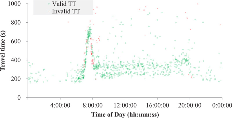
As shown in Fig. (6), the current method showed poor performance with substantial outliers unfiltered. The premise behind the current method is that the probe travel times follow the normal distribution. To verify the assumption, a normality test on probe travel times on the test section was performed. For the test, the Maximum Likelihood Estimation (MLE) for estimating parameters and the Kolmogorov-Smirnov (K-S) statistic at a 5% significance level for goodness-of-fit tests were employed. The MLE technique is generally recognized to be the best-unbiased estimator for the single distribution models that this study aims to investigate [27]. The K-S statistic, which fits a cumulative distribution to observations point by point, is considered to be the most conservative test compared to χ2 and Anderson Darling tests; in other words, it has the lowest possibility of falsely rejecting a correct fit, and for that reason, it is frequently employed by many researchers [28].
The results of the fit tests are presented in Table 1 and the relevant travel-time histogram superimposed by the distribution curves is shown in Fig. (7). The results show that the travel times do not follow the normal distribution; rather, they were correctly fitted by the lognormal distribution. This indicates that the use of the current z-score cannot be theoretically viable.
| Distribution | Number of Samples | μ | σ | K-S Statistic | Critical K-S Statistic at sig.a = 0.05 | p-value |
|---|---|---|---|---|---|---|
| Normal | 1169 | 330 | 64 | 8.85e-2 | 3.93e-2 | 1.47e-8 |
| Lognormal | 1169 | 5.19 | 0.31 | 3.66e-2 | 3.93e-2 | 0.08 |
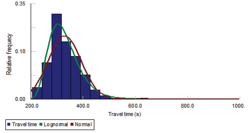
Instead, the z-score calculated from the logarithm (base e) of the travel times is justifiable. Taking these findings into consideration, a new outlier removal method is developed and will be described in detail in the section that follows.
4.3. New Technique for Outlier Removal
The proposed method expressed in Equations 4 to 7 is based on the modified z-score where the median instead of the mean as a measure of location is used. Also, the natural logarithm is applied to the raw travel times to take the characteristic of the travel-time distribution into account. The modified median filter is recognized to be resistant to abnormally deviated values compared to the standard z-score, because the median is less susceptible to the impact of abnormal values than is the mean [29, 30].
 |
(4) |
 |
(5) |
 |
(6) |
 |
(7) |
where
tt valid = valid travel times,
ln(tt i) = logarithm of travel time of i-th probe vehicle, and
z mod 99.9% = modified z-score at 99.9% confidence interval (4.45 = 3*0.6745-1).
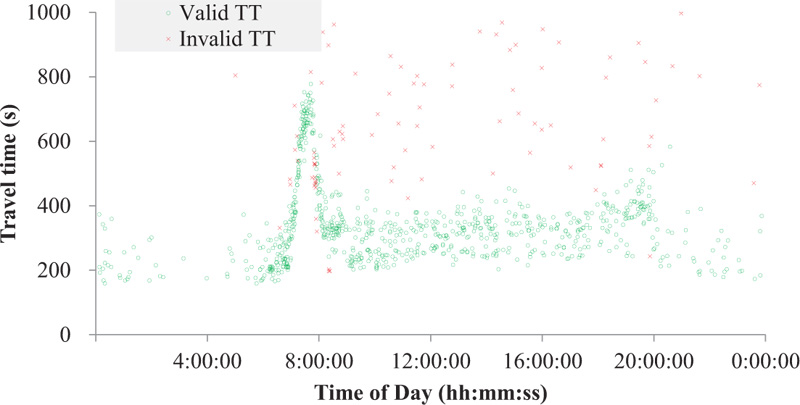
Fig. (8) shows the result of the application of the proposed method to the same data presented in (Fig. 6). Most of the outliers mainly caused by intermittent stops and round trips were properly filtered. Although some valid data were categorized into outliers, they seemingly have little influence on the travel-time information to be generated. The cleaned individual probe travel times are then aggregated into 5 min bins to be used for the prediction to reduce the time-lag in the arrival time-based travel times.
5. METHODS
5.1. Current Prediction Method
The k-NN technique is initially applied for predicting travel times on a freeway by Davis and Nihan [31]. In their model, the continuously archived probe travel times constituted the state vector as an input variable. The established model finds out k-nearest neighbors in the predefined archived travel times combined in a group (n collection intervals). The model basically assumes that the future travel times to be forecast are analogous to the past travel times in archived records. Considering repetitive human activities that produce traffic on the road, this assumption can be regarded to be reasonable. The k-NN algorithm, expressed in equations 8 to 10, constitutes five phases as described below:
1. Prepare archived travel times. For this study, month-long travel times in a 5-min bin were utilized.
2. Choose n seamlessly combined previous intervals in a group. For this study, a 30 minute-long (or six 5-min bins) travel times that exhibited the lowest prediction error for the k-NN algorithm according to an earlier study [32] were adopted.
3. Calculate the distance metric defined as the Euclidean distance and choose the number of k. The selected number of k was set at 4 based on an earlier study [25] that argued that 4 is the optimal k number considering both computing efficiency and accuracy of the model. Their rule was also proven to be valid in this study.
4. Determine k-nearest neighbors based on the calculated distance metric.
5. Predict the future travel times (the departure time-based travel times) averaged by the k-nearest neighbors weighted by the computed distance values.
 |
(8) |
 |
(9) |
 |
(10) |
where
TT(Dt) = departure time-based travel time at time t,
TTkh(Dt) = k-th departure time-based travel time at historical time t,
wk(At) = k-th weight of arrival time-based travel time at time t,
dk(At) = k-th distance between current and historical arrival time-based travel time at time t,
TT(At) = current arrival time-based travel time at time t,
TTkh(At) = k-th historical arrival time-based travel time at time t, and ,
i= aggregation interval (e.g. 5 min).
5.2. Alternative Prediction Method
The current k-NN method has been proven to be inefficient for real-time applications due to its relatively long searching time: around 2 min for 6 month-long historical data using the server system currently deployed. To improve prediction performance as well as real-time capabilities, a Recurrent Neural Network (RNN), a class of deep neural networks where connections between nodes form a directed graph along a temporal sequence, is adopted for an alternative method. Unlike the conventional feedforward neural networks, recently developed RNN models use their internal states to process sequences of inputs. This characteristic allows them to be widely applicable to tasks including handwriting recognition, speech recognition, and time-series data prediction [33, 34].
Among RNN models, a Lng Short-Term Memory (LSTM) model which can avoid the vanishing gradient problem was adopted in this study. As LSTM models are normally augmented by recurrent gates, it prevents backpropagated errors from vanishing or exploding [35]. In other words, LSTM has the merit of learning tasks that need memories of events that happened discrete time steps earlier. Also, a mix of low and high-frequency components can be handled by LSTM models [36]. All these characteristics make LSTM-based RNN models be the optimal solution for forecasting travel times in a time sequence. They can, moreover, forecast travel times on a real-time basis with less than several seconds.
The input data format, as represented in Table 2, was arranged to have a sequence length of one, a data dimension of six, and an output dimension of one. The constructed model with 10 hidden nodes was optimized by the widely-recognized adaptive moment estimation. One month-long historical data were divided into training data of 80% and testing data of 20%. The performance of the applied model is plotted in Fig. (9). For comparison with the k-NN model, six 5-min intervals data were used as independent variables where it revealed the lowest error.
| Independent Variables (Previous 30 min) | Dependent Variable | |||||
|---|---|---|---|---|---|---|
| A-25 min | A-20 min | A-15 min | A-10 min | A-5 min | A-0 min | D-0 min |
| 219 | 197 | 300 | 223 | 283 | 329 | 334 |
| 197 | 300 | 223 | 283 | 329 | 331 | 334 |
| 300 | 223 | 283 | 329 | 331 | 466 | 476 |
6. RESULTS
The significance of travel-time prediction is highlighted during peak hours because, under noncongested conditions, predicted vs. current travel times do not show notable differences. The peak hour (7-9 a.m.) probe travel times on three weekdays (Wed. – Fri.) were therefore considered for evaluation of the two prediction methods. A month-long weekday travel times on the same stretch were included in the historical database. As shown in Table 3, the average travel times on the two datasets were similar due to the recurrent travel-time patterns observed in the section during weekdays (Fig. 5).
| Item | Historical Data Set | Prediction Data Set |
|---|---|---|
| Perioda | Jan. 1st – 31st, 2019 (Weekdays) | Feb. 6th (Wed.) – 8th (Fri.), 2019 |
| Average nonpeak hour travel time | 298 s | 308 s |
| Average peak hour travel timeb | 654 s | 667 s |
bFrom 7 to 9 a.m.
Ten experiment cars were employed to collect ground truth data. The drivers were instructed to operate the cars with the floating car method where the number of cars overtaking and overtaken was equivalent. A total of 10 experiment cars with roughly 2 min headway were driven along the bi-directional roadway repeatedly during the peak hours for the three days. A total of 220 test-car runs in 75 5-min collection bins (2-4 ground-truth data in each bin) were obtained. The mean absolute error (Equation 11) was utilized to quantitatively measure the prediction errors.
 |
(11) |
where MAE= mean absolute error,
n= number of samples,
x(t)= actual (observed) travel time, and
 = predicted travel time.
Table 4 and Fig. (10) show comparisons between the ground truth and predicted travel times. In all cases, the proposed LSTM-based RNN model revealed higher performances than the current k-NN method. It also decreases the variance of prediction errors that can reduce uncertainty and therefore allows drivers to better plan activities who rely on arrival time. Further, quartile error comparisons (Fig. 11) reinforces the superiority of the proposed method where lower dispersions were observed in the alternative method.
| Statistics (s) | Wednesday | Thursday | Friday | |||
|---|---|---|---|---|---|---|
| Current | Alternative | Current | Alternative | Current | Alternative | |
| Mean | 48 | 37 | 87 | 77 | 41 | 39 |
| Variance | 48 | 29 | 105 | 69 | 48 | 32 |
| Maximum | 177 | 102 | 347 | 293 | 237 | 127 |
| 75th percentile | 65 | 45 | 115 | 132 | 52 | 50 |
| Median | 33 | 33 | 40 | 42 | 27 | 31 |
| 25th percentile | 17 | 13 | 26 | 32 | 12 | 19 |
| Minimum | 3 | 2 | 2 | 0 | 0 | 0 |


7. DISCUSSION
Although probe-based travel-time systems have merits in that they can directly collect link travel times and generally require a lower budget compared to the traditional vehicle detector-based systems, improper treatment of outlying observations and time-lag phenomenon could make them obsolete. After identifying shortcomings in the current methods, a new outlier treatment technique and an LSTM-based RNN model were proposed in this study.
To censor outliers in the probe travel times, the modified z-score that is less susceptible to aberrant values was proposed. Also, to take the characteristic of the probe travel times into consideration, the natural logarithm was applied to the raw travel times. The developed method was proven to outperform the current one. To mitigate the time-lag phenomenon, an LSTM-based RNN model, which is recently garnering much attention for forecasting time-series data is applied and its prediction performance was compared to the current k-NN method. Resultantly, it generated fewer prediction errors when evaluated by 3-day-long ground-truth data collected by test-car runs during the peak hours (7-9 a.m.) on the stretch.
CONCLUSION
Although the proposed methods were thoroughly tested on the segment, it would be preferable to be further verified through follow-up research into spatiotemporal universality by applying the proposed methods to other arterial and/or freeway systems.
CONSENT FOR PUBLICATION
Not applicable.
AVAILABILITY OF DATA AND MATERIALS
Not applicable.
FUNDING
The study is funded by the Korea Agency of Infrastructure Technology Advancement (KAIA), Korea under grant no (19 TLRP-C145770-02).
CONFLICT OF INTEREST
The authors declare no conflict of interest, financial or otherwise.
ACKNOWLEDGEMENTS
This study is the revised version of paper submitted to 2020 TRB Annual Meeting, January 12-19th Washington DC, USA.

