All published articles of this journal are available on ScienceDirect.

Travel Mode Choice Modeling: Predictive Efficacy between Machine Learning Models and Discrete Choice Model
Authors Info & Affiliations
Abstract
Background:
A complex travel behaviour among users is intertwined with many factors. Traditionally, the exploration in travel mode choice modeling has been dominated by the Discrete Choice model, nonetheless, owing to the advancement in computational techniques, machine learning has gained traction in understanding travel behavior.
Aim:
This study aims at predicting users’ travel model choice by means of machine learning models against a conventional Discrete Choice Model, i.e., Binary Logistic Regression.
Objective:
To investigate the comparison between machine learning models, namely Neural Network, Random Forest, Decision Tree, and Support Vector Machine against the Discrete Choice Model (Binary Logistic Regression) in the prediction of travel mode choice amongst Kuantan City.
Methodology:
The dataset was collected in Kuantan City, Malaysia, through the Revealed/Stated Preferences (RP/SP) Survey. The data collected was split into a ratio of 80:20 for training and testing before evaluating them between the aforesaid models. The hyperparameters of the models were set to default. The performance of the models is evaluated based on classification accuracy.
Results:
It was shown in the present study that the Neural Network Model is able to attain a higher prediction accuracy as compared to Binary Logistic Regression (Discrete Choice Model) in classifying mode choice of Kuantan users either to choose public transport or private vehicles as daily transportation. Feature importance technique is crucial for identifying the significant features in modelling travel mode choice. It is demonstrated that the Neural Network Model can yield exceptional classification of mode choice up to 73.4% and 72.4% of training and testing data, respectively, by considering the features identified via the feature importance technique, suggesting the viability of the proposed technique in supporting an informed decision.
Conclusion:
The findings highlight the strengths and limitations of the Machine Learning Technique as well as the Discrete Choice Model in modeling travel mode choice. It was shown that Machine Learning models have the capability to provide better prediction that could assist the urban transportation planning among policymakers. Meanwhile, it could be also demonstrated that the Discrete Choice Model (Binary Logistic Regression) is helpful in getting a better understanding in expressing the inference relationship between variables for improvising the future transportation system.
1. INTRODUCTION
Among all travel demand forecasting processes, travel mode choice modeling is the most critical step and one of the commonly studied areas in travel behavior research. There are many factors intertwined with travel mode choices, including a transport mode’s level of service, socio-demographic traits of users, and the attributes of the built environment associated with a journey. A deeper study on users’ daily travel mode choice, users’ preferences on transportation services, and their actual expectations on public transport that will ease the stages of the journey along the way from home to destination are essential for sustainable transportation. To develop a socially desirable and environmentally sustainable transport system in line with users’ demands, policymakers are urged to improve their understanding of users’ expectations towards public transport systems as well as variables’ characteristics associated with users’ travel mode choice [1-7].
Although a lot of improvement has been made towards the current transportation system in our country; yet users’ satisfaction with the reliability of the system is still questionable. It is important to understand mode choice since it affects the efficiency of traveling and the size of urban space required for transportation functions as well as the range of mode alternatives available for users. Current transportation planning issued by policymakers might have deviated from users’ expectations and needs; thus, travel mode choice modeling will give them a slight insight into the factors that will drive users to choose public transport in their routine. A study revealed that travel time is the most important factor that influences users’ travel mode choice compared to the other built environment and socio-demographic variables [8-10]. Users’ travel mode choice is also related to the departure time of a trip since it affected the travel time of certain modes [11].
Recently, the study on travel mode choice modeling using the application of Machine Learning Technique shows its quality for making a prediction [12-16]. Many studies prove that while comparing machine learning models with discrete choice models, they suggested that machine learning models can perform similar or higher prediction accuracy [17, 18]. Most machine learning models can learn data structures with great flexibility, as compared with logit models that practically having strict statistical assumptions [4, 8, 16, 19]. However, the logit model has an elegant closed-form mathematical structure and the ability to interpret model estimation result based on random utility theory [16, 17].
Travel mode choice modeling is not an easy task since users’ mode choice is interlocked with various factors. Over the past decades, random utility maximization theory has been widely applied for modeling travel mode choice. There are limited studies related to the application of machine learning models to predict travel mode choice, nonetheless, it was demonstrated from the studies that machine learning models could achieve at least a similar prediction accuracy against Discrete Choice models. Meanwhile, other studies achieved to establish results from the Machine Learning Technique that is substantially better [4, 7, 8]. A study conducted on mode choice for school trips by Ermagun and colleagues in 2015, revealed that the Random Forest Model achieved better results compared to the Nested Logit Model [20]. Meanwhile, a study on travel mode choice by Cheng and colleagues in 2019 depicted that the Random Forest Model performed best with a prediction accuracy of 85.36% [3]. Another study conducted by Sekhar and colleagues in 2016 Investigated the factors involved in mode choice depicted that the Random Forest model achieved higher prediction accuracy (98.96%) than the Logit Model’s prediction accuracy (77.31%) [21]. Karlaftis and Vlahogianni in 2011, reviewed the similarities and differences of analysis using Discrete Choice models against Neural Networks models in transportation research. They found that the Neural Network Model is flexible and has the power to deal with complex datasets, but in contrast, it has lacked interpretability power compared to the Discrete Choice models [22].
The objective of this paper is to evaluate the efficacy between different machine learning models against a type of Discrete Choice Model (Logistic Regression) in predicting travel mode choice among users in Kuantan City. This study is non-trivial as we shall demonstrate the development and the employment of a machine learning pipeline towards travel model choice for Kuantan City, Malaysia. We identify significant features that influence the travel mode choice. In this study, the mode of transports is classified into two main modes, namely, private vehicles and public transport. The paper is split into five parts, including Introduction, Methodology, Result and Analysis, Discussion, and Conclusion. The Introduction section provides a slight insight on factors that are correlated with users’ travel behavior and explores previous researches that perform travel mode choice modeling using machine learning technique. The Methodology section shall describe the sources of travel data as well as the different types of models evaluated as well as the performance indices employed. The Results and Analysis section shall present the prediction accuracy and provide interpretation of model estimation results. The discussion explains the significant features and the relationship with users. The Conclusion section shall summarize the findings and provides suggestions to further improve the modeling of travel mode choice.
2. METHODOLOGY
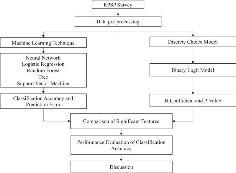
The flow chart illustrated in Fig. (1) summarizes the analysis carried out and the survey setup for this research. There are two different sections: a first section where the researchers describe models and how they work, and then a second section where the researchers explain what the case study area is, what kind of data was collected and how the data were applied in the different models.
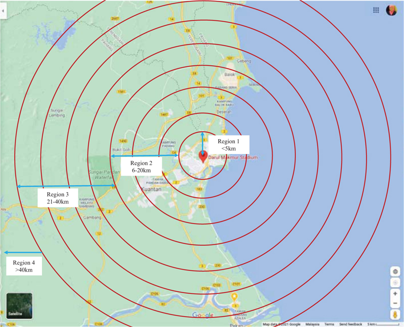
The data is collected via Revealed/Stated Preferences (RP/SP) Survey which has been conducted in Kuantan City, Pahang, Malaysia (Fig. 2). The dataset contains 1956 unique users’ preferences records, including workers, students, unemployment, retirement, and self-working. The data were saved after the data cleaning process and removal of the data trips with missing values in the dependent and independent variables. The trips were categorized into two classes, either by private vehicles (N) for both driver and passenger, or public transport (P).
The survey research was based on a quantitative approach that involves conducting a face-to-face survey with individuals. Getting information in person may be the most effective way of gaining trust and cooperation from the respondents. It is easier to react to puzzled facial expressions, answer questions, probe for clarification, or redirect responses. Face to face contact is particularly useful for detecting respondent discomfort when discussing sensitive issues or attempts to respond in a socially desirable way. The survey was conducted using Revealed and Stated Preference (RPSP) technique. This technique required the development of questionnaires that revealed users’ past experiences on using public transport, and to state their demand on current public transportation system so that they will be interested to switch mode from private vehicles to public transport.
The survey was developed by referring to the questionnaire of previous researchers and was improvised depending on the research scope and objective, which is to identify the important features that will affect users’ travel mode choice using a concept of door-to-door journey. The structure of the questionnaire was originally developed by the researchers to ease the process of interviewing the respondents. All of the questions were compressed into one page of survey form, so that the time taken to interview a user of a group of respondents can be optimized.
Users were interviewed, and their responses were recorded in the questionnaire forms. The survey was conducted in Kuantan city, including in shopping malls, shops, as well as academic institutions. The respondents were gathered in a small group of between 3 to 4 people at one time to having the short interview within 10 to 15 minutes. Some of the respondents were interviewed individually, using the same questionnaire form. There are also respondents who were having their short interview in a larger group, between 7 to 10 people at one time.
2.1. Data Pre-Processing
The variables were gathered from the literature [23, 24] as well as from the researchers’ point of view to meet the aim and the concept of research. The choice of variables was based on the theory of a door-to-door journey; where, researchers would like to understand users’ behavior on their daily travel routine and what makes them choose public transport instead of private vehicles. When making transport mode choice for a door-to-door journey, users will choose the means of transport that will get them from origin to destination the fastest and in the most comfortable and safe way. The fundamental stages included in a door-to-door journey are walking distance, waiting time, and in-vehicle time. A door-to-door journey concept is critically criticizing the method of users to embark on their daily travel starting from home to destination. Travelling using public transport consists of walking time from home to the nearest stop, waiting time at a public transport stop, in-vehicle time, and walking time from the last stop to the destination. It is important to deeply understand the behavior of users while facing the stages of a door-to-door journey using public transport so that an efficient public transportation system can be provided according to the users’ need.
Table 1 recapitulates the variables involved in the model development process, their explanation, and data sources. The dependent variables consist of users’ travel mode choice represents by public transport (bus) or private vehicles (car) either driving or passenger. The independent variables (WD1, WT, IVT, WD2) have been the main components of users’ journey starting from their origin. Other independent variables count into the dataset are total Travel Time, Ticket, Region, DOM, Age, Gender, Ethnicity, and Income.
| Variables | Explanation | Source |
|---|---|---|
| Travel mode | Travel mode (dependent variable); P=Public Transport; N=Private Vehicles | Revealed/Stated Preferences (RP/SP) Survey |
| Trip variables | ||
| • WD1 | WD1 is referred to as walking distance from home to the nearest bus stop, yet the data were presented in time (minutes). | |
| • WT | Waiting time at the bus stop. | |
| • IVT | Sitting time in the bus from pick up point until the last point users wish to be dropped off. | |
| • WD2 | WD1 is referred to as walking distance from the last stop to the destination, yet the data were presented in time (minutes). | |
| • TT | Total travel time for the whole journey starting from home until reaching the destination. | |
| Personal variables | ||
| • Ticket | Ticket price being charged for taking public transport. | |
| • Income | The users’ monthly income can be categorized as following: Income less than or equal to RM 900, income between RM 1000 to RM 2900, income between RM 3000 to RM 4900, income between RM 5000 to RM 6900, income between RM 7000 to RM 8900, and income RM 9000 and above. | |
| • DOM | DOM is a dominant factor that will affect mode choice which is suggested by users. | |
| • Gender | The sex (females/males) of users who took part in the survey. | |
| • Age | The age of users who took part in the RP/SP survey can be categorized as following: age less than or equal to 20, age between 20 to 24, age between 25 to 29, age between 30 to 34, age between 35 to 39, age between 40 to 44, age between 45 to 49, and age 50 and above. | |
| • Ethnicity | The ethnicity (Malay, Chinese, Indian & Others) of users who took part in the survey. | |
| • Region | The place where users originated from; based on the distance they traveled: | |
| Region 1: <5km Region 2: 6-20km Region 3: 21-40km Region 4: >40km |
2.2. Predictive Efficacy
The following subsection explains the details of the procedures that have been employed to look for the most convenient subset of features based on the technique called feature importance. In evaluation measurement, the comparison was made between Machine Learning Models with Discrete Choice Model.
2.2.1. Machine Learning Technique
Recent developments in the field of transportation studies have led to renewed interest in Machine Learning Technique. The application of Machine Learning Technique consists of few phases that should be followed in sequence to get a robust result. The application of this technique in modelling travel mode choice can be explored in the following sections.
2.2.1.1. Data Splitting
The machine learning models are presented by establishing the average prediction accuracy that is compared by randomly splitting the data into a training subset (80% of the data) and a testing subset (20% of the data). The prediction errors were examined as well to compare the predictive power of the feature importance by machine learning models. The total error is calculated by dividing the number of mode preferences that are predicted to have the wrong mode choice by the total number of mode preferences. Meanwhile, the mode-specific prediction error is calculated by dividing the number of mode preferences wrongly predicted from the total number of mode preferences made by that particular mode. The analysis was conducted by using Orange software; an open-source data mining tool. This software provides a set of methods and algorithms that can perform effectively in data analysis.
2.2.1.2. Cross Validation
The cross validation that is employed is the five-fold cross-validation technique to evaluate the performance of the classifiers from the training set. The importance of cross-validation is to standardise the repetition of validation and provide better insight after the data set has been reduced according to the data splitting as stated in the previous section. The fold of each iteration would give out the mean of overall accuracy and the standard deviation from each of the iterated train and test data.
2.2.1.3. Feature Importance
The technique applied to measure the importance of features was feature importance by Random Forest. The most common explanations for classification models are feature importance [25]. The term feature importance is used to describe how important the feature was for the classification performance of the model. Random Forest can be used to rank the importance of features in a regression or classification problem in a natural way.
The Random Forest algorithm has built-in feature importance, which can be computed in two ways:
a) Gini importance (or mean decrease impurity), which is computed from the Random Forest structure.
b) Mean Decrease Accuracy is a method of computing the feature importance on permuted out-of-bag (OOB) samples based on the mean decrease in the accuracy.
2.2.1.4. Machine Learning Models
Different machine learning models were investigated by incorporating the identified features, including Neural Network (NN), Random Forest (RF), Tree, and Support Vector Machine (SVM).
(a) Neural Network
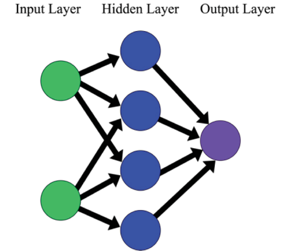
The Neural Network Model is based on the wired net of the human brain that is intended to identify patterns of given datasets [26]. It consists of several layers that stem towards the predicted outcome or responses which are made of multiple nodes interconnected with subsequent layers. The connectivity of layers between input, hidden and output works in a chain form in which the initial features or input are being intensified by the weights commonly in the hidden layer, thereby producing a distinctive input function before submitting to an activation function. Fig. (3) illustrates the structure of Neural Network model.
These artificial networks may be used for predictive modeling, adaptive control, and applications where they can be trained via a dataset. Self-learning resulting from experience can occur within networks, which can derive conclusions from a complex and seemingly unrelated set of information. In the present study, the number of hidden neurons was set to 100 per hidden layer in a two-hidden layer configuration. The Rectified Linear Unit (ReLU) activation function was also employed. The solver used in the present study is Adam.
(b) Tree
Decision trees learn how to best split the dataset into smaller and smaller subsets to predict the target value. The condition, or test, is represented as the “leaf” (node) and the possible outcomes as “branches” (edges). This splitting process continues until no further gain can be made or a preset rule is met, e.g. the maximum depth of the tree is reached.
Decision trees normally suffer from the problem of overfitting if it is allowed to grow without any control. A single decision tree is faster in computation. When a dataset with features is taken as input by a decision tree, it will formulate some set of rules for prediction.
 |
(1) |
The parameters were set as given:
a) Minimum number of instances in leaves: 1
b) Do not split subsets smaller than: 5
c) Limit the maximal tree depth to: 100
(c) Random Forest
Random Forest is a flexible, easy to use machine learning algorithm that produces, even without hyperparameter tuning, a great result most of the time. Random Forest (RF) constructs many individual decision trees at training. Predictions from all trees are pooled to make the final prediction; the mode of the classes for classification or the mean prediction for regression. However, it is comparatively slower in computation as compared to trees. Random Forest does not use any set of formulas. As they use a collection of results to make a final decision, they are referred to as Ensemble techniques. Fig. (4) depicted the structures of Random Forest in making prediction.
The parameters were set as given:
a) Number of trees: 5,
b) Number of attributes considered at each split: 5,
c) Limit depth of individual trees: 3,
d) Do not split subsets smaller than 5.
(d) Support Vector Machine (SVM)
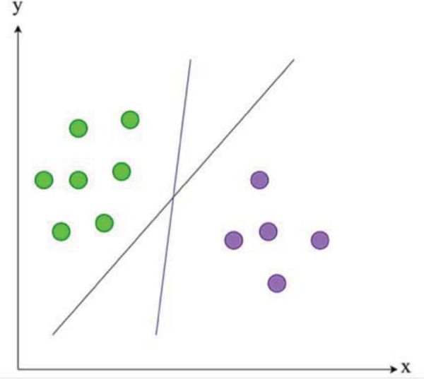
SVM is an administered learning model with related learning algorithms that break down information for arrangement and relapse examination. SVM is based on the boundaries defined by the largest distance between classes, commonly termed as margin, as visualized in Figs. (5-7). There are four basic concepts to the essence of SVM classification [27]. Firstly, the separating hyperplane. Second, the maximum- margin hyperplane. Third, the soft margin and lastly the kernel function.

These hyperplanes can be described by the equations with a normalized or standardized dataset:
With label 1, anything on or above this boundary is of one class and
With label −1, anything on or below this boundary is of the other class,
The enactment of hyperplane to isolate the classes, in this case kernel trick classes, which are being utilized in this study as the SVM algorithm, stipulates the optimal marginal distance or box constraint between these classes. The kernel function employed within a training vector to measure its performance is given in the below equation:
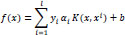 |
(5) |
The parameters were set as given:
a) SVM type with Cost (C): 0.10
b) Regression loss epsilon (ε):0.10
c) Kernel: Sigmoid tanh (gx. y+c)
d) Numerical tolerance: 0.0010
e) Iteration limit: 100
2.2.1.5. Classification Accuracy and Prediction Error
A confusion matrix is also known as an error matrix, a table that allows visualization of the performance of a classification model (or classifier) on a dataset for which the actual/predicted values of each row and column are known. Table 2 summarizes the row and column of the confusion matrices, correctly predicted choices (the diagonal cells), as well as the mischaracterized mode choice.
The confusion matrix reports the number of false positives, false negatives, true positives, and true negatives. In summary, the table yields (a) total prediction error or total error (b) the classification error or mode-specific prediction error, and (c) the percent correctly predicted or known as classification accuracy. The total prediction error is the sum of incorrectly predicted mode choices divided by the total mode choices of all modes. The classification error is the percentage of observed mode choices that are incorrectly predicted and divided by the total mode choices made by that particular mode. Meanwhile, the percent correctly predicted is the sum of correct observations found in the diagonal cells/ total true predictions divided by total mode choice of all modes. The listed metrics are important in evaluating the performance of each algorithm’s predictive power. The confusion matrix, as shown in Table 2, is an example of a binary classifier and it can be extended to the case of more than two classes. The terminology implemented in the confusion matrix can be explained as follows:
| Predicted | |||
|---|---|---|---|
| N | P | ||
| Actual | N | TN | FP |
| P | FN | TP | |
• True positives (TP): These are cases in which were predicted as yes (users will choose public transport), and users do choose public transport.
• True negatives (TN): The cases were predicted as no (users choose private vehicles instead), and users do not choose public transport.
• False positives (FP): The cases were predicted as yes, but users do not want to choose public transport. These cases are also known as a “Type I error”.
• False negatives (FN): The cases were predicted as no, but users actually will choose public transport. These cases are also known as a “Type II error”.
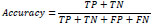 |
(6) |
2.2.2. Discrete Choice Model
Logistic Regression is a statistical method that is commonly used for any binary classification problem of Discrete Choice Models. Logistic regression describes and estimates the relationship between one dependent binary variable and independent variables.
2.2.2.1. Evaluation Measurement B-coefficient
The outcome or target variable is dichotomous. Dichotomous can be explained as there are only two possible classes, fail/pass or labeled “0” and “1”. Logistic Regression predicts the probability of occurrence of a binary event utilizing a logit function. The following basic formula depicts the general Linear Regression equation:
 |
(7) |
Where, y is the dependent variable and X1, X2,.. and Xn are explanatory variables.
Meanwhile, the Sigmoid Function can be described as following:
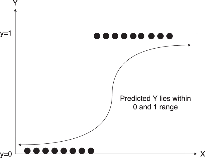
 |
(8) |
Logistic Regression is connected with utility theory, where a chosen mode is based on users’ desirability of certain variables. In other words, utility theory bases its beliefs upon individuals’ preferences, and it is widely used among economists to explain users’ behavior based on the ranking of their choices depending upon their preferences. The following equation shows the Logit Model derivation based on its sigmoid function that is applied on linear regression and is widely used in modeling travel mode choice:
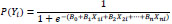 |
(9) |
where,
P(Yi) is the predicted probability that Y is true for case i;
e is a mathematical constant;
B0 is a constant estimated from the data;
B1 is a B-coefficient estimated from the data;
Xi is the observed score on variable X for case i.
2.2.2.2. P-Value
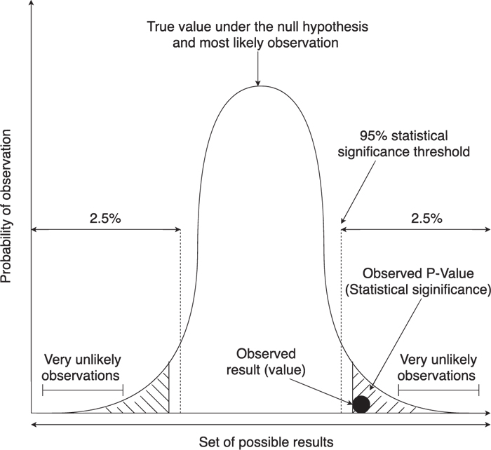
P-value or known as variables’ significant indicator is very important in statistical analysis.
The null hypothesis (H0) in statistics explained that there is no relationship between the two variables being studied. In other words, in a hypothesis developed for a case study, a variable does not have any effect on the other. In this case, any result that reflects the null hypothesis means that the results are due to chance and insignificant to support the theory being investigated. Therefore, the null hypothesis presumes that the prediction of research being studied is failed to be proved.
Once the null hypothesis is concluded to be untrue, the alternative hypothesis (H1) is adopted as the correct theory. The alternative hypothesis supports the theory that an independent variable affects the dependent variable; therefore, the results obtained are considered significant in terms of supporting the theory being investigated. The level of statistical significance is expressed as a p-value between the value of 0 and 1. The evidence is considered stronger with a smaller p-value; thus, the null hypothesis should be rejected.
A p-value less than 0.05 (or written as ≤ 0.05) is considered statistically significant. The value stipulates strong evidence against the null hypothesis. In other words, there is less than a 5% probability that the null hypothesis is correct. Thus, in such a case, researchers should reject the null hypothesis, and accept the alternative hypothesis. Meanwhile, a p-value higher than 0.05 (or written as > 0.05) is considered not statistically significant and stipulates a shred of strong evidence for the null hypothesis to be true. In this case, researchers should accept the null hypothesis and reject the alternative hypothesis.
3. RESULTS AND DISCUSSION
3.1. Descriptive Statistics
In this paper, binary travel mode choices are included in the mode choice modeling analysis for Kuantan City, which is public transport (bus) and private vehicles (car), including drivers and passengers. The total number of unique trips included in the analysis after removing missing values is 1956, among which 866 trips are made by public transport and about 1090 trips are made by private vehicles. The most common challenge encountered in modeling travel mode choices is the issue of unbalanced datasets. In this research, the majority of users choose to have travel mode choice to be made by private vehicles compared to public transport. Table 3 represents the descriptive statistics of all the variables employed in the analysis.
| - | Public Transport | Private Vehicles | - | |||
|---|---|---|---|---|---|---|
| Number of Unique Trips | 866 (44.27%) | 1090 (55.73%) | - | |||
| Independent variables | N | Minimum | Maximum | Mean | Std. Deviation | |
| DOM | 1956 | 1 | 4 | 2.09 | .806 | |
| IVT | 1956 | 4 | 270 | 38.21 | 25.443 | |
| WT | 1956 | 0 | 120 | 17.60 | 12.136 | |
| WD1 | 1956 | 0 | 51 | 7.37 | 5.110 | |
| WD2 | 1956 | 0 | 35 | 8.36 | 5.370 | |
| TT | 1956 | 11 | 325 | 71.55 | 32.761 | |
| Ticket | 1956 | .0 | 30.0 | 3.077 | 2.0224 | |
| Gender | 1956 | 1 | 2 | 1.56 | .496 | |
| Age | 1956 | 1 | 8 | 2.67 | 1.620 | |
| Ethnicity | 1956 | 1 | 4 | 1.28 | .622 | |
| Income | 1956 | 1 | 6 | 1.54 | .750 | |
| Region | 1956 | 1 | 4 | 2.67 | 1.125 | |
| Dummy variables | Number | Total | Percentage | |||
| DOM | In-vehicle time | 1 | 348 | 17.79% | ||
| WT | 2 | 1302 | 66.56% | |||
| WD1 | 3 | 96 | 4.91% | |||
| WD2 | 4 | 210 | 10.74% | |||
| Gender | Male | 1 | 858 | 43.87% | ||
| Female | 2 | 1098 | 56.13% | |||
| Age | < 20 | 1 | 222 | 11.35% | ||
| 20 to 24 | 2 | 1110 | 56.75% | |||
| 25 to 29 | 3 | 270 | 13.80% | |||
| 30 to 34 | 4 | 138 | 7.06% | |||
| 35 to 39 | 5 | 72 | 3.68% | |||
| 40 to 44 | 6 | 36 | 1.84% | |||
| 45 to 49 | 7 | 12 | 0.61% | |||
| >50 | 8 | 96 | 4.90% | |||
| Ethnicity | Malay | 1 | 1548 | 79.14% | ||
| Chinese | 2 | 300 | 15.34% | |||
| Indian | 3 | 72 | 3.68% | |||
| Others | 4 | 36 | 1.84% | |||
| Income | < RM 900 | 1 | 1110 | 56.75% | ||
| RM1000-RM2900 | 2 | 714 | 36.50% | |||
| RM3000-RM4900 | 3 | 84 | 4.29% | |||
| RM5000-RM6900 | 4 | 30 | 1.53% | |||
| RM7000-RM8900 | 5 | 12 | 0.61% | |||
| > RM 9000 | 6 | 6 | 0.31% | |||
| Region | <5km | 1 | 372 | 19.02% | ||
| 6-20km | 2 | 552 | 28.22% | |||
| 21-40km | 3 | 384 | 19.63% | |||
| >40km | 4 | 648 | 33.13% | |||
3.2. Machine Learning Results
The ablity of Machine Learning models to classify the travel mode choice was evaluated based on classification accuracy of both train and test data. The training errors of each model were also depicted to evaluate the performance of the machine learning models. In addition, the technique of Feature Importance was crucial in visualizing the significant features and to remove noises.
| Evaluated Models | Classification Accuracy (CA) | Total Errors | Mode-Specific Training Error | Mode-Specific Testing Error | ||||
|---|---|---|---|---|---|---|---|---|
| Training | Testing | Training | Testing | P | N | P | N | |
| Neural Network | 0.729 | 0.698 | 27.09% | 30.18% | 33.24% | 22.26% | 36.72% | 24.77% |
| Logistic Regression | 0.709 | 0.680 | 29.07% | 31.97% | 33.53% | 25.57% | 32.77% | 31.31% |
| Random Forest | 0.700 | 0.691 | 29.97% | 30.95% | 35.41% | 25.68% | 37.85% | 25.23% |
| Tree | 0.661 | 0.645 | 33.93% | 35.55% | 42.82% | 26.94% | 39.55% | 32.24% |
| SVM | 0.542 | 0.514 | 45.75% | 48.59% | 8.27% | 75.23% | 2.26% | 86.92% |
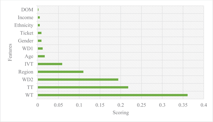
3.2.1. Feature Importance
The Feature Importance Technique was employed to find the significant features [28, 29]. Fig. (8) plots the rank of variables according to the most important until the least important of independent variables. Waiting time is the most important variable influencing users’ mode choice and it has an important measure that is far larger than other independent variables [30-32]. Total travel time is the second important variable and is followed by walking distance from the last stop to destination (WD2), Region, in-vehicle time (IVT), and Age. The other independent variables, such as walking distance from home to the nearest bus stop (WD1), Gender, and Ticket are also associated with travel mode choices. The least effect of variables on mode choice was indicated by Ethnicity, Income, and Dominant Factor (DOM).
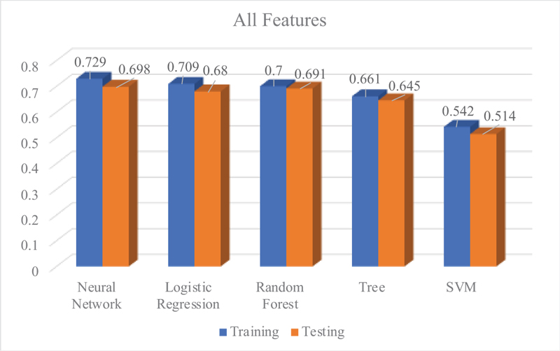
3.2.2. Prediction Accuracy of the Machine Learning Models
The result of the classification accuracy is summarized in Table 4. To compare the predictive power of the Logistic Regression Model with the other machine learning models, we also examined the training errors between modes.
As shown in Table 4, the result shows the variation of overall prediction accuracy between models, indicated that Neural Network shows the best prediction model followed by Logistic Regression, Random Forest, Tree, and SVM. The classification accuracy for the training dataset presented by Neural Network, Logistic Regression, Random Forest, Tree, and SVM is 0.729, 0.709, 0.700, 0.661, and 0.542, respectively. Meanwhile, the classification accuracy for testing datasets presented by Neural Network, Logistic Regression, Random Forest, Tree, and SVM is 0.698, 0.680, 0.691, 0.645, 0.514, respectively. Among all models, the Neural Network Model has the lowest error compared to Logistic Regression and other machine learning models. The highest error has been indicated by SVM. The Neural Network error has a total training error of 27.09% and a total testing error of 30.18%, while the Logistic Regression Model has a total training error of 29.07% and a total testing error of 31.79%. The Random Forest Model also indicated a decent error rate with a total training error of 29.97% and a total testing error of 30.95%. Meanwhile, Tree and SVM indicated the highest total training error of 33.93% and 45.75%, and testing error of 35.55% and 48.59%, respectively. Thus, the result suggested that the Neural Network Model has an overall prediction accuracy of 72.9% while the Logistic Regression model’s overall prediction accuracy is 70.9%. The rest of the machine learning models which are Random Forest, Tree, and SVM indicated overall prediction accuracy of 70%, 66.1%, and 54.2%, respectively.
As presented in Table 4, Neural Network, Logistic Regression, Random Forest, and Tree models show the highest prediction error for public transport, which is not surprising, as public transport has a much lower mode share compared to private vehicles. SVM shows the least prediction error for public transport, yet the error in predicting private vehicles is extremely high, which indicated that this model is unable to perform well while predicting travel mode choices. The training error for public transport as indicated by Neural Network and Logistic Regression is 33.24% and 33.53%, respectively. Meanwhile, the training error between these two models for private vehicles is 22.26% and 25.57%, respectively. Meanwhile, Random Forest made a fairly acceptable prediction between modes, followed by the Tree model. The poorest performance in predicting mode choice is indicated by SVM. The training error for public transport mode indicated by Random Forest, Tree, and SVM is 35.41%, 42.82%, and 8.27%, respectively, whilst the training error for private vehicles is 30.95%, 35.55%, and 48.59%, respectively. Nevertheless, Logistic Regression and the other machine learning models except for SVM indicated acceptable testing error for both public transport and private vehicles. Therefore, in this case of mode-specific prediction accuracy, both Neural Network, as well as Logistic Regression, did a decent prediction on mode choices of public transport and private vehicles compared to the other models.
3.3. Results Binary Logistic Regression Model
Table 5 tabulates the mode share and descriptive statistics from the Binary Logistic Regression Model. The model reported an acceptable goodness of fit, as the adjusted Rho-squared (Cox & Snell R-Squared) of this model is about 0.21 whilst the result is statistically significant since the p-value is less than 0.05. It indicates strong evidence against the null hypothesis, as there is less than a 5% probability that the null is correct. The descriptive statistics explained the inference relationship of variables, and the signs of all the variables included in this model are consistent with the theory.
Some of the variables of trip characteristics are significantly associated with mode choices. As indicated in Table 5, some variables are negatively associated with mode choice, which is indicated by the in-vehicle time (IVT), waiting time (WT), walking distance from home to the nearest bus stop (WD1), and walking distance from the last stop to destination (WD2). This suggests that the increase in the value of these variables would possibly cause the users to dislike using public transport. Among the variables that indicated negative association with mode choice, walking distance from the last stop to destination (WD2) and waiting time (WT) indicated the highest negative association, followed by walking distance from home to the nearest bus stop (WD1) and in-vehicle time (IVT). Users are unlikely to spend time waiting for public transport as well as walking from the last stop to the destination. Longer waiting time at the stop causes users to feel burdensome since they felt like wasting their time [33]. The same goes for walking distance from the last stop to destination (WD2), an extra walking distance caused users to feel exhausted, which in many cause the users to use another alternative of transportation to connect from the last stop to destination that will add some amount of money on their journey. In contrast, walking distance from home to the nearest bus stop (WD1) and in-vehicle time (IVT) have a more negligible effect on users’ mode choice. This scenario indicates that starting from home, users may have few alternatives to reach the nearest destination. Besides, sitting in the vehicle is usually the least factor that will influence users’ mode choice [31, 34, 35]. Users could accept having extra time sitting in a moving vehicle compared to waiting for a long moment at public transport stop [32]. The rest of the variables indicated a positive association towards mode choice, which can be explained that these variables do not affect the reduction of interest among users to choose public transport mode. However, among all variables, only walking distance from home to the nearest bus stop (WD1), waiting time (WT), in-vehicle time (IVT), walking distance from the last stop to destination (WD2), age and region indicated statistical significance in the model with a p-value less than 0.05.
The Dominant Factor (DOM) represents users’ opinion on what affects them the most that will trigger their mode choice to choose public transport or private vehicles. For example, users were questioned to pick the most important stage (variable) that they believe is the most cumbersome to them in a door-to-door journey. The variable chosen by the users was then compared with the actual reason for their decision on mode choice. The variation attributes of each variable affect users’ mode choice and at the certain condition, their decision is actually influenced by specific attributes of that particular variable, and not really influenced by the variable suggested by users at first. According to these importance scores, we are informed that the dominant factor suggested by users is deviated from what they need in a real public transportation system. The finding from this research is crucial for transportation planners and policymakers to consider users’ need while making policies in improving the services of public transportation. Barabino and colleagues in 2020 also highlighted the importance of considering users’ demand and selecting the right indicators in transit services to persuade users travelling by public transport as a daily mode [36].
3.4. Comparing Result Using Significant Features Indicated by Machine Learning Technique and Discrete Choice Model
The most important features indicated by Machine Learning Technique were waiting time (WT), total travel time (TT), walking distance from the last stop to the destination (WD2), region, in-vehicle time (IVT), and age. Meanwhile, the Discrete Choice Model was also able to indicate the important features according to P-value (p<0.05), the features of which were similar as depicted by Machine Learning Technique except for total travel time (TT). The total travel time (TT) could not be included in the utility function analysis due to the multicollinearity effect among the other independent variables.
The importance of the total travel time (TT) in estimating mode choice could be evaluated via the feature importance technique; however, it could not be included in the Discrete Choice Model due to its correlation between WD1, WT, IVT, and WD2. Thus, the Feature Importance Approach is more robust and requires minimal effort than the Discrete Choice Model, which requires rigid testing and model specification while exploring the model assumptions.
| Variables | B-coefficient | Standard Error (S.E.) | Wald | Degrees of Freedom (df) | Significance (Sig.) (P-value) | Exp (B) |
|---|---|---|---|---|---|---|
| DOM | 0.062 | 0.066 | 0.877 | 1 | 0.349 | 1.064 |
| IVT | -0.022 | 0.004 | 32.119 | 1 | 0.000 | 0.978 |
| WT | -0.065 | 0.006 | 126.794 | 1 | 0.000 | 0.937 |
| WD1 | -0.033 | 0.012 | 8.077 | 1 | 0.004 | 0.967 |
| WD2 | -0.094 | 0.012 | 65.982 | 1 | 0.000 | 0.910 |
| Ticket | 0.018 | 0.041 | 0.197 | 1 | 0.658 | 0.982 |
| Gender | 0.116 | 0.109 | 1.133 | 1 | 0.287 | 1.123 |
| Age | 0.076 | 0.036 | 4.308 | 1 | 0.038 | 1.079 |
| Ethnicity | 0.126 | 0.085 | 2.212 | 1 | 0.137 | 1.134 |
| Income | 0.062 | 0.085 | 0.530 | 1 | 0.467 | 1.064 |
| Region | 0.643 | 0.068 | 88.300 | 1 | 0.000 | 1.902 |
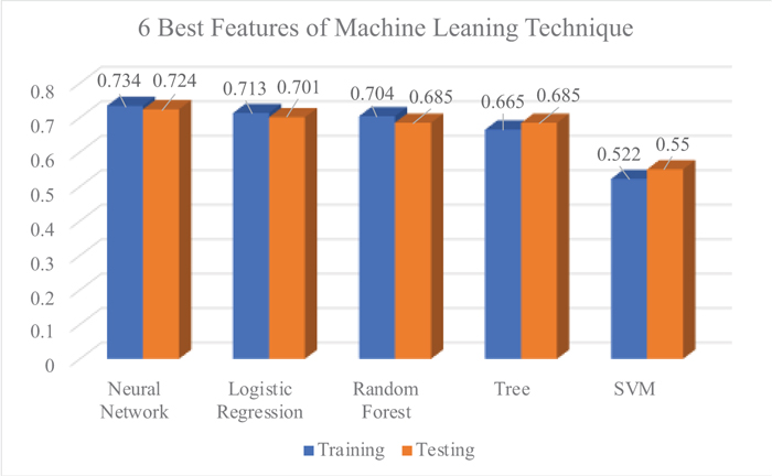
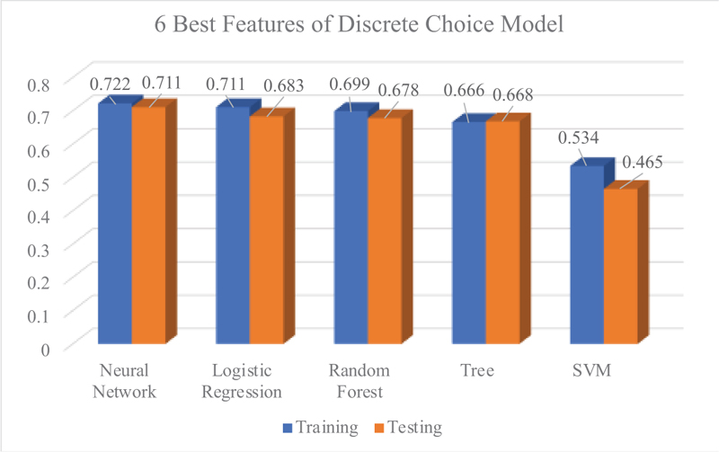
Figs. (9-11) indicated the performance of each model in classifying the travel mode choice of users in Kuantan City. The performance of the classification accuracy was compared using the best 6 features depicted by Machine Learning Technique and Discrete Choice Models. Among all Machine Learning Models, Neural Network consistently performed well in modelling travel mode choice, followed by Logistic regression, and Random Forest. As depicted in Fig. (10), the performance of the Machine Learning Models were improved after removing the insignificant features. The performance of the Machine Learning Models also improved using the features suggested by Discrete Choice Model (Fig. 11); however, the classification performance could not surpass the features suggested by the Machine Learning Technique. This technique of modelling travel mode choice can be applied in future research, to indicate the best features for prediction, by comparing the performance of models using the features depicted by both methods Table 6.
| Feature importance using Machine Learning Technique | P-Value using Discrete Choice Model |
| WT | WT |
| TT | WD1 |
| WD2 | WD2 |
| Region | Region |
| IVT | IVT |
| Age | Age |
The contribution of this study is to provide better insight regarding the method of modelling travel mode choice using Machine Learning Technique and Discrete Choice Model. The result of this study is in line with the findings from previous researchers [19] and [16] that Machine Learning Technique provides better performance in predicting travel mode choice, since it had a pipeline of method to indicate the best features for making prediction. However, some models applied were different from other research and the goodness of that model in predicting the travel mode choice is varied depending on the type of dataset being used.
In this paper, Neural Network is presented as the best model in prediciting travel mode choice from dataset conducted using RPSP Survey. Other researchers [19] suggest that Neural Network performed well in predicting travel mode choice from a dataset collected using Socio-economic Panel Survey Liewen zu Le ̈tzebuerg (PSELL Survey). Meanwhile, others depicted Machine Learning Models can produce significantly higher prediction accuracy than logit models using Stated-Preference (SP) Survey [16]. Future research should investigate other Machine Learning Models and tune the hyperparameter of each model to find out their performance in predicting travel mode choice.
CONCLUSION
Travel mode choice modeling is a crucial step in travel demand forecasting. The present study has compared the efficacy of machine learning models as well as Discrete Choice Model (Binary Logistic Regression) in forecasting travel mode choice in Kuantan City, Malaysia. The significant features that influence mode choices were explored via features identified by the Discrete Choice Model as well as the Feature Importance Approach of Machine Learning, as reported in the previous section. It was shown that the Neural Network Model could predict the mode choice reasonably well. Future studies shall investigate the effect of the identified features on different machine learning models. The effect of tweaking the hyperparameters of the model shall also be investigated. The present study is non-trivial towards relevant stakeholders in transportation studies in general as it provides insight into the efficacy of machine learning models in predicting travel mode choice.
CONSENT FOR PUBLICATION
Not applicable.
AVAILABILITY OF DATA AND MATERIALS
The data supporting the findings of the article is available from corresponding author [N.F.M.A.] upon reasonable request.
FUNDING
This study is funded by the Graduate Assistant Scheme by Universiti Sains Malaysia, Pulau Pinang, Malaysia.
CONFLICT OF INTEREST
The authors declare no conflict of interest, financial or otherwise.
ACKNOWLEDGEMENETS
Declared none.

