All published articles of this journal are available on ScienceDirect.

Semi and Nonparametric Conditional Probability Density, a Case Study of Pedestrian Crashes
Abstract
Background:
Kernel-based methods have gained popularity as employed model residual’s distribution might not be defined by any classical parametric distribution. Kernel-based method has been extended to estimate conditional densities instead of conditional distributions when data incorporate both discrete and continuous attributes. The method often has been based on smoothing parameters to use optimal values for various attributes. Thus, in case of an explanatory variable being independent of the dependent variable, that attribute would be dropped in the nonparametric method by assigning a large smoothing parameter, giving them uniform distributions so their variances to the model’s variance would be minimal.
Objectives:
The objective of this study was to identify factors to the severity of pedestrian crashes based on an unbiased method. Especially, this study was conducted to evaluate the applicability of kernel-based techniques of semi- and nonparametric methods on the crash dataset by means of confusion techniques.
Methods:
In this study, two non- and semi-parametric kernel-based methods were implemented to model the severity of pedestrian crashes. The estimation of the semi-parametric densities is based on the adoptive local smoothing and maximization of the quasi-likelihood function, which is similar somehow to the likelihood of the binary logit model. On the other hand, the nonparametric method is based on the selection of optimal smoothing parameters in estimation of the conditional probability density function to minimize mean integrated squared error (MISE). The performances of those models are evaluated by their prediction power. To have a benchmark for comparison, the standard logistic regression was also employed. Although those methods have been employed in other fields, this is one of the earliest studies that employed those techniques in the context of traffic safety.
Results:
The results highlighted that the nonparametric kernel-based method outperforms the semi-parametric (single-index model) and the standard logit model based on the confusion matrices. To have a vision about the bandwidth selection method for removal of the irrelevant attributes in nonparametric approach, we added some noisy predictors to the models and a comparison was made. Extensive discussion has been made in the content of this study regarding the methodological approach of the models.
Conclusion:
To summarize, alcohol and drug involvement, driving on non-level grade, and bad lighting conditions are some of the factors that increase the likelihood of pedestrian crash severity. This is one of the earliest studies that implemented the methods in the context of transportation problems. The nonparametric method is especially recommended to be used in the field of traffic safety when there are uncertainties regarding the importance of predictors as the technique would automatically drop unimportant predictors.
1. INTRODUCTION
Vehicle crashes are among the leading causes of death around the world, where annually, more than 1 million people die, and more than 20 million are severely injured [1]. Vehicle crashes are ranked 7th in terms of causing mortality [2], which is equivalent to more than $230 billion worth of crash costs every year. A significant proportion of those crashes are related to pedestrian crashes, where the pedestrian is defined as any person being not in or on a motor vehicle [3].
Despite the efforts and success in reducing crash fatality in general, the number of pedestrian fatalities has increased from 14% of the fatality decomposition in 2009 to 20% in 2018, which is equivalent to 6,283 deaths [4]. To reduce the high number of deaths due to pedestrian crashes, the first step could be to identify the leading factors ofthose crashes.
Studies were conducted to identify factors that contribute to pedestrian crashes and the next paragraph outlines a few of them. The study was conducted to analyze contributory factors to the severity of pedestrian-bus crashes [5]. Some of the identified important factors include darkness, location of crashes, speed zone, and age of the pedestrian. The associated factors to the severity of pedestrian crashes were analyzed [6]. Intersection proximity, lighting condition, type of vehicle and its speed, and pedestrian impairment were some of the important factors. In another study, some of the factors to the severity of pedestrian crashes were pedestrian characteristics, environment factors, and crash characteristics [7]. A partial proportional odds model with threshold heterogeneity by the scale and proportional odds factor was used for modeling pedestrian crashes [8]. The results highlighted that drivers under influence, type of vehicles, estimated speed of vehicles, and driving over the recommended speed are some of the factors contributing to the severity of pedestrian crashes.
On the other hand, policy attention has been given to the identification of the parameters’ estimates in a most accurate way so appropriate countermeasures could be employed. Parametric and nonparametric approaches have been implemented in the literature review to achieve the objective. Application of nonparametric method could overcome the shortcoming of potential pitfall of parametric misspecification, which might preclude valid reference by using a wrong distribution, which the model does not adhere to.
Various methods have been proposed to identify the distributions of the parameters. One of the most popular and simple ways for estimating the distributions is through the frequency approach: splitting the samples into bins and counting how many samples fall into each bin. However, although the traditional method could be a good representation for probability mass function, it could not be a representative for probability density function (PDF); unless we shrink the bins of the histogram by using more data observations. To address the shortcoming of the histogram, the kernel method could be employed, which could address the histogram shortcoming by providing smooth density across all points: better performance is expected when the smoothing parameter goes to zero but slower than 1/n.
Due to the strength of the kernel method, especially for multivariate models, the semi and nonparametric methods are often based on an extension of simple kernel density or conditional kernel density. For instance, given various explanatory variables of crashes as X, such as weather or road conditions, what would be the estimated conditional density of y given X, which is based on both vectors of X and Y. Still, some of the challenges of the conditional kernel density are what the optimal smoothing parameters are, and whether all the parameters are relevant to be included in the model or not [9].
Although extensive studies were conducted in the literature review for modeling crash severity, the majority of those studies, for instance, implemented parametric specification, assume the distribution error term to be limited to normal or logistic. However, past studies highlighted that the parametric method of logit or probit models, for instance, could be severely biased as the distribution of the error terms might be heteroscedastic or asymmetric [10].
Also, not as many studies have been conducted in the literature with the help of non- or semi-parametric kernel-based methods in the field of traffic safety, so few studies in other areas would be highlighted here. Parametric and semi-parametric estimation, including single index, for binary response model, was used. The analyses were conducted on different datasets. The results highlighted while in one study, the probit model outperformed the semi-parametric approach; in another dataset, the semi parametric was superior.
A combination of categorical and continuous variables was considered for a case study in the literature [11]. The study considered the implementation of the nonparametric kernel-based estimator. The smoothing parameters were obtained from the cross-validation and minimizing the integrated square error (ISE). The results highlighted that the proposed method performs highly better than the conventional nonparametric frequency estimator. For instance, the employed method highlighted a better performance than the probit method on a simulated dataset based on a confusion matrix. It should be noted that in that study, the least-square cross-validation selection was used for smoothing parameters.
Nonparametric estimation of the regression function with both categorical and continuous data was used in another study with the kernel method [12]. It was found that the out-of-sample squared prediction error of the proposed estimator for that study is only 14-20%. The study examined the relationship between governance and growth using a nonparametric method [13]. The findings highlighted the significance of attributes and the relationship between growth and governance.
A semi-nonparametric generalized multinominal logit model was formulated using orthonormal Legendre polynomial to extend the standard Gumble distribution [14]. The model was implemented on commute mode choice among alternatives or travel behavior. The results of the implemented model highlighted that the method violates the standard Gumble distribution assumption, which would result in inconsistency in parameters estimates.
The semiparametric single-index model for estimating the optimal individualized treatment strategy was applied [15]. The results highlighted the suitability of the technique for the objective of the study. In another study, the semiparametric method originated from the single-index methodology was used. The study addressed the challenges of the standard single index model, where observed data are biomarker measurements on pools rather than individual specimens [16].
A potential methodological shortcoming of the parametric methods is that they assume that the model follows some parametric functional form. So, it is expected, if the model is mis-specified, the results of the estimations might be misleading, and consequently, it would not be the right representation of the dataset.
The contributions of this manuscript are as follows:
● There is no certainty that implemented traditional statistical methods would follow some predefined distributions, the conditional probability density is employed non-parametrically using cross-validation for bandwidth selection, with an objective function of minimizing mean integrated squared error (MISE).
● As the main advantage of the implemented nonparametric method is to adjust the bandwidth for parameters based on their relevancies, we discuss the selection of bandwidths by considering the standard and noisy data for our model.
● In addition, as semi-parametric method, parametric method was used for a comparison purpose. The performances of the incorporated models were evaluated using confusion matrices.
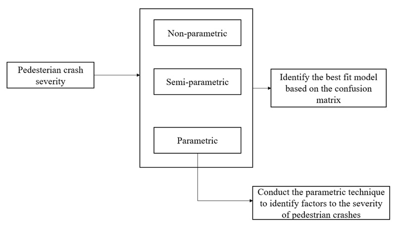
The flowchart of the implemented steps is depicted in (Fig. 1).
As can be seen from the figure, while we compare the performance of the model based on 3 techniques, the parametric method would be used to highlight important predictors.
The remainder of this manuscript is structured as follows: the method section will discuss in detail the two main implemented methods. Then the data section would describe the data being used in this study. The results section would be presented into 3 subsections. First, the considered models would be compared in terms of confusion matrices. Then the model parameters estimates would be discussed. In the last subsection, we will present the model performance in bandwidth adjustment for the removal of some predictors. The conclusion section will summarize the findings.
2. METHODS
For the kernel estimation method, contrary to other parametric methods, we assume that the samples are drawn from an unknown density function and the goal is to estimate the density function from the observed dataset. The method sections would be presented into 2 main subsections. First, a general background would be presented, followed by the kernel-based nonparametric method. Finally, we will present a semiparametric estimation of the Single Index Model. It should be highlighted that both methods can be implemented on our dataset, incorporating both discrete and continuous attributes.
2.1. General Background
Although the traditional kernel method has mostly assumed the underlying data is continuous, in many cases, especially in transportation problems, the data might include categorical or binary attributes. Traditionally, in case of having both continuous and categorical data, the frequency approach would be implemented, where the data would be categorized into cells being assumed for categorical data, and then the density approach would be implemented on the continuous attributes in each cell.
However, the frequency approach is expected to perform unsatisfactorily as it would result in efficiency loss due to the employment of the sample splitting method, especially in the case of having a large sample size. Therefore, a kernel-based estimator could be employed for any type of dataset, categorical or a mixture of both continuous and categorical, to address the shortcoming of the frequency method as it does not rely on sample splitting [17].
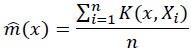
We start with a univariate kernel density function for continuous and discrete variables, then expand it to our methods. The kernel function for the continuous attribute could be written as:
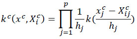 |
(1) |
Where k is the kernel function, Xcij are univariate independent and identically distributed samples drawn from some unknown distributions at a point of xjc. h is called smoothing parameter, bandwidth or window width. It is intuitive from the above equation that when the smoothing parameter of h is too large, the important features would be obscured [18].
On the other hand, the kernel for discrete variables could be written as:
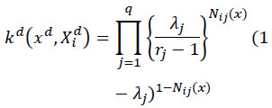 |
(2) |
Where λq are smoothing parameters for discrete attributes. While the boundary of 0 < hj < ∞, the boundary of λj is 0 ≤ λj ≤ (rj-1)/rj, where rj is number of categories of a discrete variable. So, in the case of having a binary attribute, the maximum of λj would be 0.5. In other words, while in case of being an unrelated attribute for a continuous attribute, hj → ∞ for categorical variable and in case of binary predictor λj → 0.5, making a binary attribute to be an unrelated attribute.
While using any nonparametric method it should be noted that the inclusion of the parameters that are independent of the response should be removed before conducting any statistical analysis as not excluding the irrelevant attributes would degrade the parameters’ estimate accuracy and prediction. The problem of irrelevant attributes in the nonparametric setting could be alleviated by choosing smoothing parameters. The cross-validation technique could be implemented by simultaneously choosing smoothing parameters for attributes and thus removing irrelevant explanatory components [9]. It would be implemented by extending the irrelevant attributes’ bandwidths to infinity and thus eliminating irrelevant attributes. The cross-validation could be based on the simplest form of minimization of least-square for selection of the smoothing parameters [19] or other methods.
2.2. Kernel-Based Nonparametric Method
This subsection is based on the work in the literature [9]. The objective function is to identify smoothing parameters that minimize the MISE as:
 |
(3) |
Where hp and λq are bandwidths for the continuous components and smoothing parameters for the discrete components, respectively. Recall, 0 < hp < ∞, and 0 ≤ λq ≤ (rj - 1)/rj, where xd takes values of 0, 1,…, rj-1. xc is p-variate, while xd is q-variate. m is a marginal density and m(x) = m c(X c| X d) P (X d = x d). It is intuitive from Equation 3 that the objective function is mainly based on minimization of the expected variation between the expected conditional density. g
g (y | x) highlights the density of y conditional on x, which could be written as g (y | x) = f (x,y) / m(x) while g
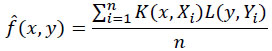 |
(4) |
 |
(5) |
Where K and L are generalized kernels. Comparably, K for considering both continuous and categorical would be written as:
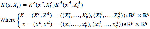 |
(6) |
X, as the whole explanatory variables, which could be split into X= (xc, xd), where x c and x d accommodate continuous and discrete predictors, respectively. L, which was used in 4, would be changed accordingly based on y and Y in L (y, Yi)
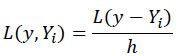 |
(7) |
For this method, cross-validation would be used to overcome challenges of incorporating attributes that seem to be irrelevant and included in the model. It would be implemented by assigning large smoothing parameters and shrinking the parameters to the uniform distribution so they would not be considered in model performance.
Obtaining the optimal values of smoothing parameters for various attributes, the MISE needs to be minimized. The MISE in 3, and after considering the above equations, could be extended to [9]:
 |
(8) |
Where X is a function including dominant terms of MISE, where “a” and “b” are functions of h and λ, and n is the number of observations. For instance, h j = aj n(-1 / p + 5), or λj = aj n(-1 / p + 5). In summary, the parameters, such as smoothing, would be identified by minimizing X or MISE, by having constrained the parameters to be non-negative. It should be noted, for instance, that X, in addition to being a function of all ap and bq, it is also a function of the second derivative of f (xc, xd, y) with respect to y.
Equation 8 is also based on “ud” . “ud”, compared with x d, being only different from attributes in jth components, in case of the component having no information regarding the response. In other words, in case of irrelevant information, the jth component would be removed from xc, or xd. For estimation of MISE, and as expected, due to the multivariate nature of the algorithm, in the process of X every pairwise consideration of xc, ud given y, f (xc, ud, y), m (xc, ud) and f (x, y) would be considered. The interested readers are referred to the literature review for more description [9].
The following paragraphs will outline a single index model or semiparametric estimation. Besides nonparametric method, the semiparametric method of the single-index model was considered in this study. The description of the semiparametric single index model in this subsection is based on the work in the literature [10]. The method, the functional form of the choice probability function, is characterized by an index, and thus the model makes no assumption regarding the distribution or generating the disturbance. The method has been discussed for the binary choice model only as:
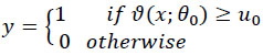 |
(9) |
where ϑ in ϑ (x; θo) is a known function with x as a vector of exogenous variables, and θo as an unknown parameter vector, and uo is the random disturbance. The model is called the index restriction model, as E (y | x) is restricted to E (y | ϑ (x; θo)), where E is the conditional expectation, and ϑ (x; θo) is an index. uo from above could be written as uo ≡ s(x; βo). ε, where s is the positive scaling function known, and other parameters were defined earlier. uo highlights the known heteroscedasticity of a known form of s(x; βo) and heteroscedasticity of unknown ε being independent of x.
Now, maximum likelihood could be employed to estimate θo in 9 as:
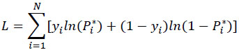 |
(10) |
It should be noted that Equation 10 looks similar to the binary logit model with the difference that ln (Pi*) and ln (1 - Pi*) would be estimated. Where Pi* could be written as:
 |
(11) |
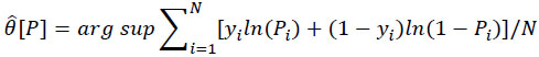
Where Fu|x is a known cumulative density function (CDF). To simplify further, while assuming u and x are independent, Fu|x could be written as Fu. Now, Fu would be maximized by θ jointly. However, still, the distribution function might be replaced by its maximum likelihood estimate. Thus Pi*(θ) would be replaced by P(θ), which is tractable and could locally approximate Pi*(θ).
After doing some algebra, the objective function process would be transformed to estimate θ by minimizing the Kullback-Leibler information criteria (KLIC), or discrepancy between θ
 |
(12) |
The above is based on the fact that the known probability function of P performs asymptotically similar as Q(P
In summary, Pi*(θ) in 11 is replaced with tractable Pi(θ) in 12, which could be locally approximated. That starts from constructing Pi(θ) by using C as the event u < v (x; θ), so Pi*(θ) in 11 would be written as P*[v(x; 0); 0] = Pr[C]gv|c(v; θ) / g(v; θ), which could be replaced by Co, which is an event C at θo, or uo < ϑ(x; θo) equivalent for y=1 in Equation 9.
As a result, we could write p(vo; θo) based on probability of y=1, conditioned on various explanatory variables, Pr[y=1|x]. So, the analysis would be employed on the proportion of pedestrian crashes that result in severe crashes.
2.3. Data
The models described above were applied to a case study of the pedestrian crash dataset in Wyoming. The data consists of a sample of pedestrian crashes that occurred in Wyoming during 2010-2019. The dataset was directly obtained from the Wyoming Department of Transportation (WYDOT). The considered attributes in Table 1 are based on their significance in parametric analysis. Table 1 highlights that across all considered variables, only posted speed limit is continuous. The characteristics are all related to pedestrian crashes and the mean highlights the distribution of those pedestrians involved in crashes. For instance, the pedestrian’s gender could be divided into almost equal proportions, mean=0.43.
3. RESULTS
This section will be presented in 3 subsections. First, the performance of the three models in terms of accuracy will be presented. The second subsection would compare the parameters estimates of the semi-parametric and parametric methods. In the last subsection, noisy attributes would be added to the nonparametric technique to see how the model handles the noisy attributes by choosing appropriate smoothing parameters.
3.1. The Models’ Performance
This section is conducted to compare the performances of the implemented methods. As semi- and nonparametric methods are not based on log-likelihood, standard measures such as the Akaike information criterion (AIC) are not suitable for comparison. As a result, the performances are evaluated by means of confusion matrices. To address the concern that the methods have seen the used data, we split our data into two subsets of the test and training dataset and the confusion matrices of both datasets are presented in Table 2. It should be noted that only the correct classification rate (CCR) of the test data is considered and presented in Table 2.
About 14% (No=100) of balanced observations randomly were assigned for the test dataset, while the remaining (No=711) were used to train the model. The numbers are chosen due to limited observations and a balanced vision about the model performance on the test dataset. As can be seen from Table 2, the accuracy for the training dataset is 75%, 68%, and 67% for nonparametric, semi-parametric, and parametric methods, respectively.
However, as it is possible that the methods were overfitted, it is more reliable to look at the models’ performance for the test dataset. The model performance on the test dataset highlights that the nonparametric method outperforms the other method by 79% accuracy compared with 71% and 77% for semi-parametric and parametric methods, respectively. The severe crash prediction is of crucial importance for policymakers ofthe state as reduction of injury or severe crashes is aparamount priority. As can be seen from Table 2, CCR (1) has the superior performance for semi-and nonparametric methods, 76% and 68%, respectively. So, semi- and nonparametric methods especially work better than the parametric method on the category of pedestrian severe crashes.
The performance of the included models is in line with the work in the literature review that the nonparametric method would outperform the semi- and parametric counterparts [20]. Finally, it should be noted that another study was conducted to investigate the pedesterian crash severity.
Although nonparametric was able to adjust itself for both test and training datasets, both semi- and parametric methods perform largely better than the parametric method over the training dataset. More studies are needed, especially in traffic studies, to confirm the findings.
| Attribute | Mean | Variance | Min | Max |
|---|---|---|---|---|
| Response, no physical damage 0, minor or functional disability injury 1 | 0.55 | 0.248 | 0 | 1 |
| Non-level grade as 1 (vs others*) | 0.17 | 0.141 | 0 | 1 |
| Straight ahead maneuver as 1 (vs others*) | 0.46 | 0.249 | 0 | 1 |
| Alcohol involvement as 1 (vs others*) | 0.18 | 0.145 | 0 | 1 |
| Location of 1st harmful even being on shoulder (vs others *) | 0.15 | 0.127 | 0 | 1 |
| Drug was involved in the crash (vs others*) | 0.03 | 0.055 | 0 | 1 |
| Posted speed limit, continuous | 50 | 5,577 | 15 | 90 |
| Pedestrian gender, female as 1 (vs male*) | 0.43 | 0.245 | 0 | 1 |
| Lighting condition, Night as 1 (vs others *) | 0.36 | 0.231 | 0 | 1 |
| Nonparametric Method | Semi-Parametric Method | Parametric Method | |||||||
|---|---|---|---|---|---|---|---|---|---|
| PDO | Non-PDO | PDO | Non-PDO | PDO | Non-PDO | ||||
| Test | PDO | 45 | 5 | 33 | 17 | 46 | 4 | ||
| Non-PDO | 16 | 34 | 12 | 38 | 19 | 31 | |||
| Training data | PDO | 287 | 32 | 196 | 123 | 266 | 53 | ||
| Non-PDO | 147 | 245 | 101 | 291 | 183 | 209 | |||
| Test | % Correct | 79% | 71% | 77% | |||||
| dataset | % CCR (0) | 90% | 64% | 92% | |||||
| % CCR (1) | 68% | 76% | 62% | ||||||
| Model Parameters | Parametric Method | Semi-Parametric Method |
|---|---|---|
| Intercept | -1.63 | - |
| Non-straight maneuver | 0.76 | 1 |
| Night lighting condition | 0.46 | 0.101 |
| Non-level grade | 0.88 | 0.192 |
| Alcohol involvement | 0.82 | 0.159 |
| Location of crash being off roadway | 0.46’ | 0.084 |
| Drug involved in the crash | 0.86’ | 0.058 |
| Female pedestrian | -0.33” | -0.051 |
| Posted speed limit, continuous | 0.031 | 0.005 |
| 1st model | 2nd model | |||
|---|---|---|---|---|
| Attributes | Bandwidth | Maximum lambda | Bandwidth | Maximum lambda |
| Non-straight maneuver | 0.14 | 0.5 | 0.20 | 0.5 |
| Night lighting condition | 0.29 | 0.5 | 0.10 | 0.5 |
| Non-level grade | 0.28 | 0.5 | 0.09 | 0.5 |
| Alcohol involvement | 0.0001 | 0.5 | 0.2 | 0.5 |
| Location of crash being off roadway | 0.006 | 0.5 | 0.09 | 0.5 |
| Drug involved in the crash | 0.006 | 0.5 | 0.499 | 0.5 |
| Female pedestrian | 0.27 | 0.5 | 0.12 | 0.5 |
| Posted speed limit, continuous | 2.02 | 5.10 | 4.33 | 8.73 |
| Driver age, discrete | - | - | 5.9 | 6 |
| Non dry road condition | -- | -- | 0.101 | 0.5 |
| Downhill roadway area | -- | -- | 0.20 | 0.5 |
3.2. Models’ Parameters’ Estimates
As the nonparametric method is not dealing with parameters’ estimates, distributions, and related bandwidths, and parameters’ estimates could not be obtained. As a result, the point estimates of semi- parametric and parametric are only included in Table 3. Although most parameters are significant at the 0.05 significance level based on the binary logistic model, it should be noted that the two variables were significant at 0.1 level only, and the p-value was .19 for an attribute of pedestrian gender for that model.
For both models, the estimations are in line and have expected signs. For semi-parametric, based on design, the first attribute is normalized to 1. Comparison across the parameters’ estimates magnitudes is not recommended as the parametric method incorporates an intercept, and the first attribute of the semi-parametric is normalized to 1. However, across both models, alcohol and drug involvement, driving on non-level grade, and bad lighting conditions are some of the factors that increase the likelihood of pedestrian crash severity.
3.3. Nonparametric Bandwidth Adjustment for Handing Noisy Attributes
To have a vision about the bandwidth estimates of the model attributes and to see if any irrelevant variables have been removed from the analysis by assigning upper bandwidth close to the maximum value, Table 4 is provided. Table 4 presents the maximum and assigned bandwidth values for continuous and categorical variables. For the nonparametric method, cross-validation automatically identifies irrelevant and relevant components and diverges the irrelevant to infinity so the distribution would be virtually uniform on the real line [9].
In simple words, the process would be summarized as follows: first uniform priors, or initial parameters values, would be given to the parameters, where λ is close to 0.5. Then the probability estimates would be updated by seeing observations, wherein case of λ being close to 0, the prior would be updated based on the samples, while in case of λ → 0.5, the uniform prior, or initial value, would be the estimated value of the parameter. Recall that for categorical attributes λj ≤ (rj - 1) / rj.
It is clear that a larger variance is associated with those λ being closer to 0, while a smaller variance, or larger bias, is related to those λ being closer to 0.5. When bandwidth is close to a maximum value of λ, there is proof that the parameter distribution is flat with a variance of almost zero, so the parameter is irrelevant in the model.
Two models were included in Table 4. First, the model, which we discussed in the results of previous subsection. We also added some noisy variables, such as driver age, in a continuous format to the second model. From the first model in Table 4, the nonparametric method even took advantage of those variables that were based on the parametric method found to be associated with uncertainty and not being different than 0: for instance, the bandwidth of pedestrian gender is 0.27 compared with a maximum value of 0.5. So, the attribute was kept in the model.
Moving to the second model, we incorporated noisy attributes. As can be seen from the second model in Table 4, a wider bandwidth closer to the maximum values is given to driver age. A wider bandwidth has been given also to the drug involved attribute. Previously based on Table 3, there was an uncertainty for this attribute based on the logit model. Although the attribute was kept in the first model, when adding some noisy attribute, this predictor was removed from the dataset. The other variable is a discrete attribute of pedestrian age. The nonparametric method has done a good job in giving a wide bandwidth close to the maximum to this value, so the distribution for this attribute would be flat, and thus this attribute would be considered irrelevant, see the second model in Table 4.
4. DISCUSSION
Pedestrian crashes are a matter of great importance for policymakers and safety engineers in Wyoming due to their high severity rate. Pedestrian crashes have been primarily studied in the literature in the parametric framework. However, it is likely that the error terms’ distribution following traditional distribution would be unrealistic. In other words, the assumption that the model follows preassigned distributions would result in an unjustified restriction. Thus, this study was conducted to evaluate the performance of semi- and nonparametric methods in the evaluation of pedestrian crash severity.
One of the challenges of the kernel-based model is its process in the estimation of mixed discrete and continuous variables, which is common for traffic studies datasets. The two semi- and nonparametric methods use kernel estimation techniques, minimizing the assumption made about the underlying probability density. Two main methods, being mainly based on the kernel method, were employed to compare the performances of the models by checking their predictabilities. The cross-validation approach, in the nonparametric method, would use optimal smoothing parameters, which asymptotically minimize the cost function of the mean integrated squared error through using optimal values for smoothing parameters. It could be done by using optimal values for important attributes and removing irrelevant components by assigning a large smoothing parameter.
To have a fair comparison, the models’ parameters were prescreened. Therefore, initially, no variable was removed from the nonparametric technique. However, to have a vision about best performed model, or the nonparametric method, a few unimportant attributes were incorporated in the model in another analysis to see how the bandwidth would vary to exclude those irrelevant attributes. Recall, bandwidths parameters would be estimated to minimize the objective function of MISE.
In order to examine the goodness of fit of employed models, confusion matrices were considered. The nonparametric method outperforms both parametric and semi parametric methods in accurately predicting the pedestrian crash with 79% accuracy compared with 71% and 77% for semi-and parametric methods. It is worth discussing that the non- and semi-parametric methods performed well in correctly predicting the outcome of severe crashes. Due to prescreening process, the nonparametric method did not use its capability of adjusting the bandwidths for irrelevant attributes. However, still, the method outperformed the other two methods.
As there is no parameter for the nonparametric method, the parameter estimates of logit and semi-parametric were used for comparison. It was found that the estimated coefficients do not vary significantly across the semi- and parametric methods, especially in terms of their signs or magnitudes.
It should be noted while doing analysis it was noticed that the nonparametric method is especially expected to perform well when there are uncertainties associated with some attributes. While making any conclusion, the lack of enough observations, especially for the test dataset, should be taken into consideration. For this study, based on the parametric method and by considering only very important parameters, p-value<0.01, it was observed that the performance of the logit model would be improved. That might be due to the fact that the nonparametric method is expected to perform superior, especially due to removal of irrelevant attributes. Again, the results of this study are specific to the dataset being used. More studies needed to highlight the strength and shortcomings of the included kernel-based methods, especially for transportation problems.
CONCLUSION
In summary, a few important points were observed from the implemented techniques. The nonparametric method is recommended to be employed in traffic safety study for prediction when there are uncertainties about the importance of some predictors as the method would discard unimportant predictors. More studies are needed to assess the applicability of the employed techniques. In terms of the findings, alcohol and drug involvement, driving on non-level grade, and bad lighting conditions are some of the factors that were found to increase the severity of pedestrian crashes.
CONSENT FOR PUBLICATION
Not applicable.
AVAILABILITY OF DATA AND MATERIALS
Not applicable.
FUNDING
None.
CONFLICT OF INTEREST
The authors declare no conflict of interest, financial or otherwise.
ACKNOWLEDGEMENTS
Declared none.

