All published articles of this journal are available on ScienceDirect.
In-tunnel Accident Detection System based on the Learning of Accident Sound
Abstract
Introduction:
Traffic accidents are easy to occur in the tunnel due to its special environment, and the consequences are very serious. The existing vehicle accident detection system and CCTV system have the issues of low detection rate.
Methods:
A method of using Mel Frequency Cepstrum Coefficient (MFCC) to extract sound features and using a deep neural network (DNN) to learn sound features is proposed to distinguish accident sound from the non-accident sound.
Results and Discussion:
The experimental results show that the method can effectively classify accident sound and non-accident sound, and the recall rate can reach more than 78% by setting appropriate neural network parameters.
Conclusion:
The method proposed in this research can be used to detect tunnel accidents and consequently, accidents can be detected in time and avoid greater disasters.
1. INTRODUCTION
The increase in tunnel accidents has become an important issue as the number and length of tunnels have also been increased due to many mountains' geographical characteristics and the human pursuit of low time and inexpensive transportation costs [1]. Because of narrow space and tunnel vision, secondary accidents often occur, so the consequences of tunnel accidents are more serious than ordinary roads [2]. There are three characteristics of tunnel accidents. First of all, it is difficult to rescue the accident in the tunnel. Secondly, tunnels are prone to fire, and the number of casualties is more than that of ordinary roads [3]. Finally, the tunnel is not bypassed and is heavily blocked. So tunnel accident detection system is more important than the general road traffic management system.
There are numerous defects in the current accident detection system. Vehicle accident detection system has a high error detection rate [4]. There is high computational complexity in video detection, and it takes a lot of time [5]. CCTV manual detection will have some visual impairment area and needs a lot of time. CCTV Image Processing algorithm proposed in the paper [6] uses GMM to determine the amount of change in pixels and first detects the stationary vehicle due to an accident in the tunnel. But it also has the problems of complex calculation and low detection rate. In order to solve the above problems in the existing technology, a tunnel accident detection method based on acoustic signal is developed, which is not only low cost but also considerably advantageous in detection rate and detection speed.
The purpose of the paper is to develop an Accident Sound Detection (ASD) algorithm by identifying tunnel accident sounds to detect traffic accidents as early and accurately as possible and prevent secondary accidents. Because the tunnel accident sound is the subcategory of abnormal sound, and it is not a human voice, the development of abnormal sound recognition technology lags behind that of speech recognition technology. At present, most of the extraction methods of abnormal sound features draw experience from the field of speech recognition. So the feature extraction method used is to borrow the widely used MFCC feature extraction method [7, 8]. The MFCC coefficients, MFCC delta coefficients, and MFCC delta-delta coefficients are used as the input data of the follow-up neural network sound detection system. Then the deep neural network [9, 10] with strong learning ability and classification ability is used to classify accident sound and non-accident sound. Although we focus on the accident sound of the tunnel, our method can also be applied to the classification of other abnormal sounds. The ASD proposed in the paper can recognize the accident sound by learning the accident sound data of the selected tunnel. Moreover, it can continuously improve the performance by accumulating increased data based on time.
2. METHODS
The sound data with hiddenness of parameters and features cannot be directly classified. The sound data need to be preprocessed and their feature extracted. Preprocessing can remove the invalid part of the original sound and construct training samples containing valid sound information. Then, features representing sound information are extracted. This chapter will explain the preprocessing, feature extraction methods, and selected classifier.
First of all, the actual accident sound and non-accident sound are obtained, and the sound library is established. Second, the sound is preprocessed. What's more, the main features are extracted from the preprocessed sound. Finally, the obtained sound features are used for classifier learning. To adjust the parameters of the classifier is to predict the sound category more accurately. The structure of the sound classifier is shown in Fig. (1).
2.1. Sound Library
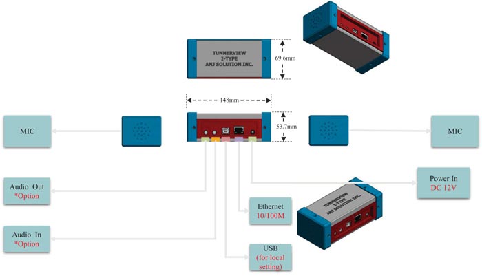
Experimental data is sound data collected from actual tunnels. The sound collector used includes MIC, audio input, output, Ethernet link, USB power, and other parts. The size of the entire device is about
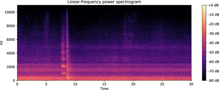
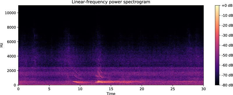
From November 2018 to April 2019, total 3343 sounds were detected, and each sound file was 30 seconds. We call these sounds abnormal sounds. After watching and listening to CCTV, the company staff classifies abnormal sounds into 14 classes of sound types. The statistics of sound classes are shown in Fig. (3). The sound library is built through the already acquired 3343 tunnel sound data and the number of new occurrences in the future. Because clash sounds are the object of our attention, we divide each sound file into accident sounds and non-accident sounds. The accident sounds include clash sounds, and the other 13 sounds are non-accident sounds. Figs. (4 and 5) show examples of spectrograms of an accident sound and a non-accident sound. The spectrogram is obtained by dividing a long sound signal into frames, adding windows, and then performing fast Fourier transform for each frame. After that, the results of each frame are stacked along another dimension to get a picture. The horizontal axis represents time, the vertical axis represents frequency, and the brightness of color represents amplitude.

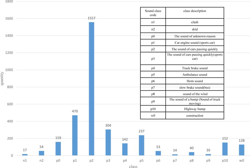
It can be seen from Fig. (3) that there are only 17 accident data and 3326 non-accident data. Due to the serious imbalance between the accident and non-accident sounds, the accident sound data needs to be augmented. The augmentation method is to compose a new accident sound by the accident sound and several non-accident sounds.
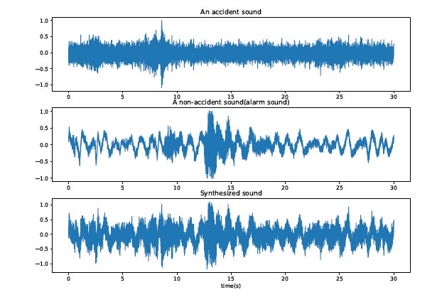
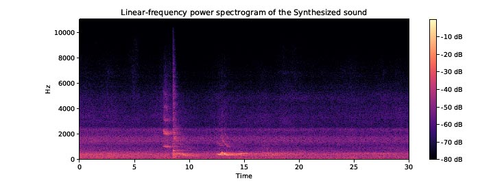
For example, the accident sound in Fig. (4) and the alarm sound in Fig. (5) are combined to produce a synthesized sound. Fig. (6) is their time-domain diagram. From the time-domain diagram, we can see that although the noise is not reduced after the sound is combined, the time-domain characteristics of the original sound still exist. Around the 8th second in the accident sound and around the 13th seconds in the alarm sound, these peaks (the moment when there is an abnormal sound) all appear on the synthesized sound. Fig. (7) is the spectrogram of the synthesized sound, and we can see that the synthesized sound still has the frequency characteristics between the two sounds. Obviously, such a combination method helps to augment the accident sound data of the experiment and helps the learning of the classifier.
2.2. Pre-processing
Because preprocessing affects the features to be extracted and then affects the classifier's performance, sound preprocessing is crucial. Preprocessing of existing sound signals involves channel conversion [11], resampling [12], pre-emphasis, framing, windowing, and Voice Activity Detection (VAD).
2.2.1. Channel Conversion
Different input sound collectors result in different numbers of input sound channels. If it is stereo, we need to convert it to mono.
2.2.2. Resampling
Depending on the collector or its settings, the sample rate of the sound may vary. Higher sampling rates are used for data resampling. In our experiments, 48000 Hz is selected.
2.2.3. Pre-emphasis
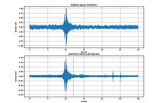
It can be seen from Fig. (4) that the accident sound is present in the high-frequency components because the high-frequency components in sound signals are more easily absorbed and blocked [13]. Pre-emphasis processing on sound signals can effectively supplement high-frequency components in sound signals. The Pre-emphasis can also reduce noise interference indirectly. Its function is usually implemented by using a first-order FIR digital filter [14]:
 |
(1) |
where x(t) is the signal after resampling. α is the pre-emphasis weight. xpre-emphasis(t) is the signal after pre-emphasis. Fig. (8) shows the results of the time domain before and after the pre-emphasis of an accident sound. It can be seen from the figure that some parts of the signal have been enhanced and the noise is weakened.
2.2.4. Framing and Adding the Window
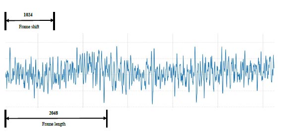
The sound signal is a time-varying signal that is stable for a short time [15]. A short and stable sound clip can be used as a frame. This frame is intercepted from a fixed characteristic continuous sound. This process is called framing [16]. In order to ensure the smoothness between frames and the continuity of sound signals, it is usually processed by overlapping frames. In human voice recognition, the length of each frame is between 10ms and 40ms, and the frame shift size is usually half of the frame length. If the framing is too short, there will be an insufficient frequency domain. If the framing is too long, the signal will be unstable, and the frequency domain conversion will become worse. The accident sound is the sound of a clash, which generally lasts for a long time. After our experimental test, it has a good performance when we select 2048 signal sampling points (about 42ms) as the frame length and 1024 signal sampling points (about 21ms) as the frame shift. An example of framing is shown in Fig. (9).
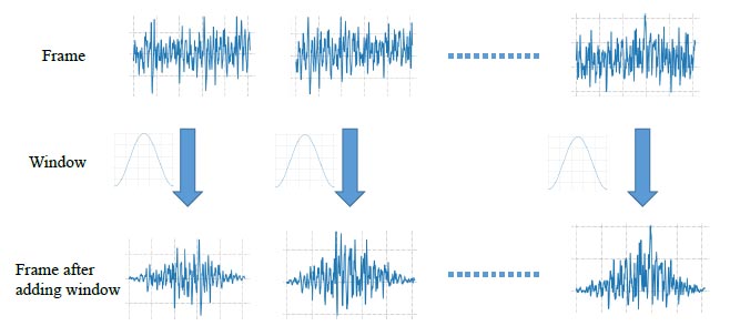
In order to keep the smoothness of each end of the frame, sound frames are windowed. The process of windowing is shown in Fig. (10). Windows are usually a rectangular window, Hanning window, and Hamming window [17]. The window function as follow:
 |
(2) |
(2) where w(n) is the window function. M is the length of the window. When α is 0, the window is the “rectangular window”. As the value of α is 0.46, the window is the “Hamming window”. And α is 0.5, the window is the “Hanning window”.
2.2.5. Voice Activity Detection
Voice activity detection method can accurately find the start and end positions of a sound signal and obtain a sound segment that can accurately represent sound information. The use of VAD not only improves the voice detection rate but also reduces the amount of computation [18]. There are many VAD methods, and we choose the most commonly used detection method based on energy and average zero-crossing rate [19]. The obtained sound material is an accident sound that is intercepted for 30 seconds from each sound file. As can be seen from Figs. (4 and 5), not all sound signals are useful. Abnormal signals are shown at about 8 seconds in Fig. (4), and 10 seconds, 13 seconds in Fig. (5). Through the VAD method and setting the appropriate threshold, each file can intercept the signal of an appropriate number of frames as a valid signal. However, not all the signals intercepted in the accident sound are accident sound signals, and it is also possible to intercept non-accident sound signals in the accident sound. Therefore, these sound clips need to be re-labeled after VAD. We only need to re-label the clips intercepted by the accident sound in our work because the non-accident sound does not contain the clash sound.
2.3. Feature Extraction
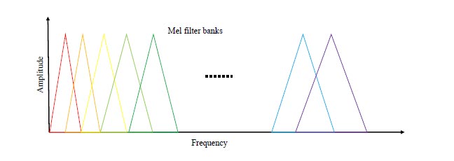
Although the MFCC feature extraction method was originally used to extract human voice features, later, it has been proved that it exerts a good effect on the extraction of environmental sound features [20]. Because the tunnel sound has the characteristics of environmental sound, MFCC can be used to extract the feature of abnormal tunnel sound. The reason why MFCC is chosen is that it has the advantages of dimension reduction and decorrelation [21]. The dimensionality is reduced because the number of sampling points per frame is reduced from 2048 to 20-dimensional MFCCs. Decorrelation is changed from time correlation in the time domain to no correlation in the frequency domain. The process of MFCC feature extraction is shown in Fig. (11). As shown in Fig. (12), the Mel filter banks have different responses to the traditional linear spectrum and the Mel spectrum [22]. Mel filter banks are placed at regular intervals according to the proportion of Mel. In the Mel frequency domain, sound detection is linear. Since the width of all filters is similar to the human hearing threshold bandwidth, it can simulate human hearing. The extraction process of MFCC is as follows [14, 23]
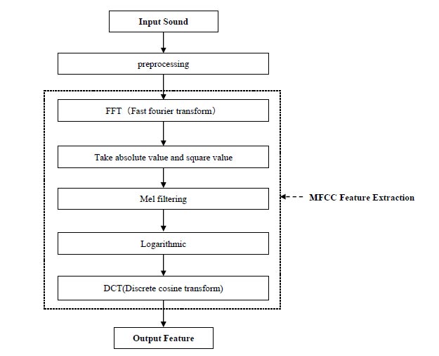
(1) The frequency spectrum of each frame is obtained by the fast Fourier transform.
(2) The power spectrum is obtained by taking the absolute value and square value of the spectrum.
(3) Pass the power spectrum through a set of Mel scale triangular filter banks, typically 40 filter banks.
(4) Calculate the logarithmic energy of the output of each filter bank.
(5) MFCC coefficients are obtained by Discrete Cosine Transform (DCT).
In our method, although the final cepstral coefficients of each frame were 40, 20 were retained, and the rest were discarded. The reason for discarding the other coefficients is that they represent fast changes in the filter bank coefficients, and these fine details do not contribute to sound detection. These 20 values are called MFCC features. If we use ƒi to represent the i -frame, then the difference between the MFCC features of ƒi+1 and the MFCC features of ƒi are called delta coefficients. The difference between the delta coefficients of ƒi and the delta coefficients features of ƒi+1 are called delta-delta coefficients. Both of them reflect the information of the sound in the dynamics.
2.4. Learning
Deep Neural Network (DNN) has proven to be a powerful model for sequence information such as computer vision and natural language processing [24]. With the deepening of the research on neural networks, the application scope of speech and sound through neural networks is also expanding [25].
The fully connected neural network is a typical forward neural network, which is representative of the artificial neural network [26]. It usually contains multiple hidden layers, and the neurons between adjacent layers are fully connected. However, neurons between the same layers are not connected. The multi-layer neural network has been fully proved to have the function of completing the complex nonlinear mapping and has played a great role in the field of pattern recognition [27].
The feature that we extracted is not a simple linear relationship. We choose DNN as the classifier, map the extracted features to the space of other dimensions, and use the activation function to establish a nonlinear relationship. Finally, backpropagation is used to adjust the network parameters and optimize the loss function. With MFCC features as input, the classification results can be obtained more accurately.
The confusion matrix [28] structure of our classifier is shown in Table 1.
| - | Predicted class | ||
|---|---|---|---|
| - | Accident Sound | Non-accident Sound | |
| Actual class | Accident Sound | TP | FN (Type I Error) |
| Non-accident Sound | FP (Type II Error) |
TN | |
There is a problem that is worthy of our attention. If the experimental data class distribution is uneven, there will be a learning problem [29]. For example, suppose the ratio of accident sound data to non-accident sound data in the training data is 1:9. In that case, if all the prediction results are non-accident sound, the accuracy will still reach 90%. This shows that accuracy is not usually the preferred performance measure of classifiers. In such an imbalanced data set, recall represents the proportion of real accident sounds predicted as accident sounds. Because our goal is to find the accident in time, so it is most important. Accuracy represents the overall performance of the model. So we choose these two performance measures to evaluate the experiment.
The Accuracy is calculated as:
 |
(3) |
The Recall is calculated as:
 |
(4) |
Type I error indicates that the accident sound is predicted to be a non-accident sound, which is a very serious problem because it may cause the accident to go undetected and result in loss of life and property. The increase of type I error will decrease recall value, which is inversely proportional to each other. Type II error indicates that the non-accident sound is predicted to be the accident sound, which results in an increase in the burden on the tunnel workers and more work. Obviously, the type I error is more important than the type II error. It would be nice if the values of type I error and type II error could be reduced at the same time, but this is not the case, and they affect each other to some extent. Therefore, we should use the improved loss function to improve the prediction ability of the model.
 |
(5) |
where α is a coefficient that we can specify.
 is the predicted result of the i -th data, ti is the target of the i-th data.
3. RESULTS AND DISCUSSION
The experiment runs on a Windows 10 operating system, the CPU is Intel i5-7600, and the memory is 16GB. The computer language is python3.6. Programming experiments are performed on the software Pycharm 2018.1. The main python libraries are numpy, keras, ffmpeg, librosa, etc.
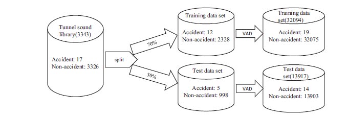
The sound sampling rate set in this experiment is 48000Hz. First of all, accident sound and non-accident sound are split into a training data set and a test data set according to the proportion of 7:3. Then the sound files of the training data set and the test data set are preprocessed, respectively. Each frame's size is 2048 sampling points, and three frames are taken as a sample by VAD. A total of 46011 experimental data samples were generated after VAD processing. After manually labeling the data samples again, there are 33 tunnel accident sounds and 45978 non-accident sounds in the data. The split process of test data and training data in specific experiments is shown in Fig. (13).
We will augment the accident data with augmentation methods. Although some accident sound data was added by using this method, it is still not enough. Therefore, accident sounds and non-accident sounds were selected for training in a certain proportion during the experiment. The data is prone to over-fitting or the phenomenon that most of the data is predicted to be a class with a high proportion. The result may be that the test data's accuracy is very high, but the recall is very low.
In Fig. (14), we denote the MFCC feature vectors of the three frames as M1, M2, and M3, respectively. We use the following two different methods to get the final sound feature vector.
(1) Method 1 is to combine the MFCC feature vectors of 3 frames, and the final feature vector is
(2) Method 2 is the MFCC features of the first frame, the delta coefficients, and the delta-delta coefficients, so the final feature vector is
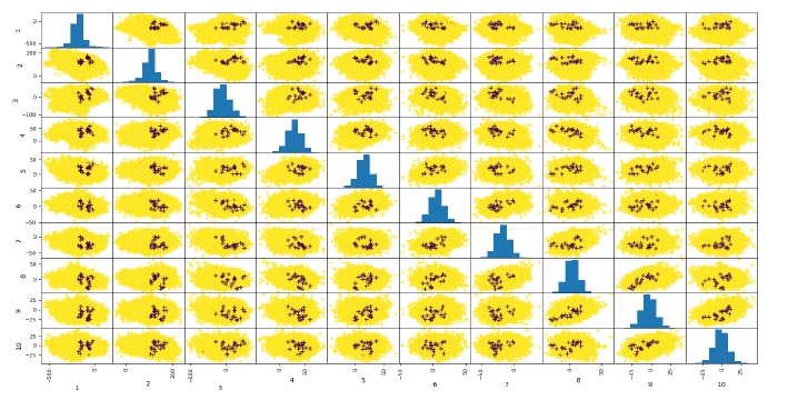
Fig. (15) shows the distribution of the first 20 features of the 60-dimensional features extracted by method 1. It is found that the relationship between the features is not obvious. So we need to learn the neural network to find the relationship between features.

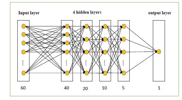
The neural network used in our experiment is a fully connected neural network, and its structure is shown in Fig. (16). In fact, I conducted a lot of choices on the number of neural network layers and nodes in my experiment were seen. For example, the number of hidden layers is 5, and the number of nodes is 200, 100, 50, 20, 5, respectively. And found that as long as it is not extreme, similar results can be obtained. The input layer is the MFCC feature extracted, and the hidden layer uses the Relu activation function. The only node in the output layer represents the predicted result. And the output layer uses the sigmoid function, which ensures that the input result is between 0 and 1. If its value is close to 0, the prediction result is accident sound. On the contrary, if its value is close to 1, the prediction result is non-accident sound. The optimization method is the Adam algorithm [30]. The loss function uses the mean squared error function [31]. Our models use mini-batch gradient descent to learn, and the batch size is 200. The learning rate is 0.002, and the number of training times for each model is 5000 times.
The final experiment is an orthogonal experiment with two variables. Variable one is the amount of accident sound augmentation, and variable two is the ratio of accident sound to non-accident sound. We used method 1 and method 2 to do two sets of experiments. The experimental results on the test data are shown in Figs. (17 and 18). Abscissa α indicates that the ratio of accident sound to non-accident sound in the training data is 1: α . The vertical coordinates of each line of figure from left to right are accuracy and recall, respectively. The blue line indicates that a “general experiment” means that the sound is not augmented. The orange line “augmentation 5”, the gray line “augmentation 10” and the yellow line “augmentation 20” are the augmentation of the accident sound by 5 times, 10 times and 20 times, respectively. Compared with method 2, method 1 has better performance in accuracy. However, in method 1, we can see that the recall rate is very variable. That is because sometimes the model performs well on the training data, but may not perform well on the test data. As shown in Figs. (17 and 18), as the alpha value increases, the accuracy of each method roughly increases. This is because the accident sound is not balanced compared to the non-accident sound, resulting in a certain degree of overfitting.
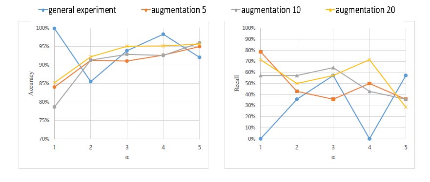
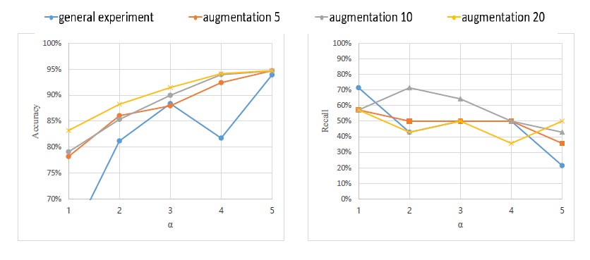
As can be seen from Fig. (17), when the ratio of accident sound to non-accident sound is 1:1, and when there is no sound augmented, the recall is about 78%. This is due to 14 accident sounds and 13903 non-accident sounds in the test data. And the amount of data used in training is not very sufficient, resulting in the result of low learning effect. In future work, we will collect more accident sound data to improve the learning ability of the classifier. It can be seen from Fig. (13) that the ratio of accident sound and non-accident sound in the test data is 14:13903. Therefore, 78% of the accident sound can be detected from so many abnormal accident sounds. This shows that our method is effective.
Table 2 compares the running speed of our experiment. They are the average results of 100 experiments. The time of feature extraction refers to the time consumed in the stage of single 3-frame sound data from reading to extracting the 60-dimensional feature vector. The time of model prediction refers to the time it takes to predict after a single 3-frame sound feature is extracted. The time of 3 frames of sound is about 85ms (4096 sampling points). But we predicted it took less than 5ms. It proves that our algorithm can detect accident sounds extremely quickly. High detection speed will have a beneficial influence on the application of our algorithm to real-time detection.
| Methods | Time of Feature Extraction | Time of Model Prediction | Total Run Time |
|---|---|---|---|
| Method 1 | 4.7347ms | 0.0020ms | 4.7367ms |
| Method 2 | 4.9426ms | 0.0021ms | 4.9447ms |
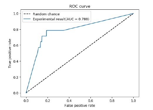
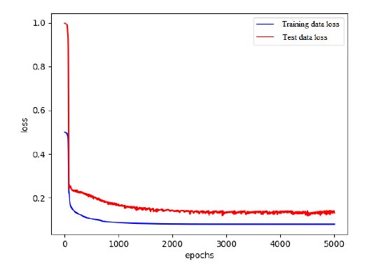
The experimental data results with the highest recall rate to make the ROC figure and the figure of loss value were used. Fig. (19) shows the ROC curve of the test and the calculated AUC score. The calculated AUC scores were 0.788, so it can be seen that the proposed method produces good results for the classification of accident sound data sets. Fig. (20) shows the average loss function values of the training set and test set. In the figure, we can see that the model converges quickly and performs well on the dataset.
CONCLUSION
Accident detection is a very important problem in the tunnel. Compared with vehicle accident detection systems and video detection, sound detection has the advantages of low cost and fast detection speed. In the present paper, we proposed a tunnel accident sound classification algorithm based on MFCCs feature and deep learning model. MFCC features extraction method is not only fast but also obtains high-quality and low-dimension features. The deep neural network is used as the classifier model because it has a good ability for continuous learning. With the increase of accident sound data collection in the tunnel, its learning ability and detection rate will become better and better in the future. Under the condition of serious imbalance class distribution of current data, we design a method to balance the data and adjust the class weight. The experimental results show that in the case of a serious lack of accident sound, the recall can reach more than 78%. In our future research, we will comprehensively use video detection, sensor detection, and sound detection in the tunnel to determine whether an accident has occurred in the tunnel. We will also focus on the real-time acquisition and detection of tunnel sounds to achieve real-time monitoring.
CONSENT FOR PUBLICATION
Not applicable.
AVAILABILITY OF DATA AND MATERIALS
The data and materials used to support the findings of this study are available from the corresponding author (L.Y.) upon reasonable request.
FUNDING
None.
CONFLICT OF INTEREST
The authors declare no conflict of interest, financial or otherwise.
ACKNOWLEDGEMENTS
Declared none.

