All published articles of this journal are available on ScienceDirect.

Deep 3D Dynamic Object Detection towards Successful and Safe Navigation for Full Autonomous Driving
Abstract
Background:
Infractions other than collisions are also a crucial factor in autonomous driving since other infractions can result in an accident. Most existing works have been conducted on navigation and collisions; however, fewer studies have been conducted on other infractions such as off-road driving and not obeying road signs. Furthermore, state-of-the-art driving models have not performed dynamic 3D object detection in the imitation learning stage; hence, the performance of such a model is unknown. No research has been conducted to investigate the driving models' computational complexities.
Objective:
The objective of this research is to study the effect of 3D dynamic object detection for autonomous driving and derive an optimized driving model with superior performance for navigation and safety benchmarks.
Methods:
We propose two driving models. One of them is an imitation learning-based model called Conditional Imitation Learning Dynamic Objects (CILDO), which performs dynamic object detection using image segmentation, depth prediction, and speed prediction. The other proposed model is an optimized model of the base model using an additional traffic light detection branch and deep deterministic policy gradient-based reinforcement learning called Conditional Imitation Learning Dynamic Objects Low Infractions-Reinforcement Learning (CILDOLI-RL).
Results:
An ablation study proves that using image segmentation and depth prediction together to enable three-dimensional object vision improves navigation performance rather than taking decisions entirely from the image. The CILDOLI-RL model presented in this paper achieves the highest score for the newly introduced No-Other-Infraction benchmark and No-Crash benchmark. It scores a moderate score for the Car Learning to Act (CARLA) benchmark in both the training town and the testing town, ensuring safe autonomous driving. The base CILDO model achieves the best performance in navigation and moderate scores for safety benchmarks under urban or rural dense traffic environments in both towns. Both proposed models are relatively computationally complex.
Conclusion:
For safety-critical driving, since both navigation performance and safety are crucial factors, it can be concluded that the proposed CILDOLI-RL is the best model out of the two proposed models. For applications where driving safety is not of much concern, the proposed CILDO is the best model.
1. INTRODUCTION
1.1. Background
1.1.1. Traditional Approaches
Autonomous driving and navigation have been a problem that people have been trying to solve for the past three decades. Several attempts have been made to recognize a pattern in sensory inputs to map into driving functions. The early solutions had been more biased towards heuristic approaches, in which decisions for navigation were provided to the robot using algorithms [1]. These systems can be considered a modular pipeline consisting mainly of three pipeline stages: perception, local planner, and continuous controller in order. In such systems, the sensor data is provided to a perception module which then plans the motion by generating way-points or detecting lane edges to decide the next state and finally to provide a control algorithm to get the desired navigation function for the robot [2].
In a study [3], a SONAR-based crop row mapping technique is used, which is a row following technique along with fuzzy logic control for navigation. Proportional Integral and Derivative (PID) control for the steering of a tractor had been used with the help of geomagnetic sensor readings [4]. Some researchers have used image processing techniques to extract features from cameras to aid in making navigation decisions. In a study [5], this technique was used in an agricultural environment, where crop row lines were extracted from raw camera images using the morphological image and threshold functions, which is a row following technique. These techniques can be considered edge/line detection techniques to aid driving decisions.
Sensor data fusion is another key research area in autonomous navigation systems, where the fusion process directly affects the outputs of the system, which are the actions of the robot. Kalman filter has been extensively used in traditional systems for autonomous driving due to its robustness to multisensory noise [6]. Recent work shows that particle filter performs better than Kalman filter for navigation in orchards [7]. This classical approach involves the use of Simultaneous Localization and Mapping (SLAM) [8] using the Kalman Filter, graphs, particle filter, and monocular visuals.
1.1.2. Modern Approaches
A more recent approach is to aid machine learning in autonomous navigation. Machine learning has been used for computer vision, a sub-system in modern autonomous driving. Specifically, a traditional modular pipeline is constructed with the help of Convolutional Neural Networks (CNNs), which recognize patterns in sensor data [9]. Similar to crop row or lane identification using image processing techniques, modern approaches use Recurrent Neural Networks (RNNs) for the same task, but with advancements such as the detection of lanes using a stack of images that can overcome partial sensor observations [10]. Some use only CNNs for real-time semantic segmentation with bounding boxes considering the fast inference [11]. A modular pipeline involves a separate perception module that can be optimized using depth, semantic features and a driving module, where perception from computer vision is used to obtain driving functions, such as controlling throttle and steering [9].
Another approach is using imitation learning, which is a supervised learning approach. It involves either a trained human or a robot performing tasks, which are then imitated by a learner to find a policy to map a given state to a set of driving actions [12] by detecting patterns in input data. Even though the concept of application of imitation learning for autonomous driving runs back to the late 1990s [13], it had gained recognition in the recent past due to advancements in Deep learning. Originally, imitation learning for autonomous driving has been trained using the DAGGER (Dataset aggregation) algorithm [12]. An online imitation learning system for off-road autonomous driving has proven to perform better than batch imitation learning systems. In a study [14], authors proposed an additional execution layer to ensure safety and feasibility by tracking the short-term trajectories extracted from the policy layer, formed by a small neural network trained using imitation learning. However, this study is limited to vehicle following, lane following and overtaking on straight roads and does not address complex urban driving scenarios. In another study [15], the bird’s view of the driving environment is used for imitation learning to get the driving policy integrated with a safety controller and a trajectory tracking module to ensure safe driving. The use of RNNs for imitation learning based on crowd-sourced video data is also presented in a study [16]. A more recent approach is to use conditional imitation learning, a blended version of the conventional modular approach with imitation learning for high-level end-to-end driving while responding to low-level intermediate commands (Ex: route commands) as conditions between end-to-end driving during test phases [17]. This work removes the error due to the assumption that sensory perception alone contributes to taking driving actions in end-to-end driving. This system provides alternative paths to get to the same location, which agrees with the practical scenarios. The conditional imitation learning system does not do end-to-end mapping of a given state directly to steering and throttle. It maps the state (camera readings) to intermediate features to be fused in an intermediate layer and provided to the control layer for controlling function [17, 18]. These conditional imitation learning approaches provide better results than the preceding end-to-end training method.
Reinforcement learning is another one of the major research areas for autonomous driving. Reinforcement learning is an unsupervised learning approach, where an agent in a given state takes action to maximize future rewards obtained from the environment. It has been used for lane following in high curvature roads [19]. In a study [20], depth information of the monocular cues is mapped for steering direction control using reinforcement learning to avoid obstacles. Driver assisting cooperative adaptive cruise control system with vehicle-to-vehicle communication for longitudinal control of vehicles using reinforcement learning to optimize the control policy has been used [21]. As a sub-problem of autonomous driving, reinforcement learning has been used for overtaking decision-making on highways using Q learning [22]. Another sub-problem is automatic lane changing that can change lanes even under unforeseen instances using reinforcement learning [23]. A study demonstrated [24] how reward functions for deep reinforcement learning can be designed considering collision, keeping in lane, speed, distance to goal etc. Moreover, in another study [25], the authors investigated how DRL can be used to effectively learn how to pass occluded intersections and overcome heuristic approaches. The camera vision is encoded into a latent state, and then a deep Q network agent is trained [26] to obtain a model-free deep RL. In multi-fidelity reinforcement learning, the policies for low-fidelity simulators are transferred to high-fidelity simulators for exploring heuristics to find optimal policies with fewer data [27]. A constrained Markov Decision Process (MDP) called survival-oriented RL, which takes survival (Negative avoidance) as the first priority rather than maximizing reward, is considered [28] for ensuring safety. Multi-Agent RL has been used for high-level strategic decision-making, such as overtaking and following vehicles using dynamic coordination graphs [29]. Despite the super-human performance of reinforcement learning in gaming environments, a study [30] examined the requirement for a deep deterministic policy gradient algorithm to cater to complex and continuous state, action space in autonomous driving. A deep RL framework for autonomous driving using sensor fusion and RNN is also presented [31].
1.1.3. Motivation
In the literature on autonomous driving, it has been mentioned that a total heuristic system mapping sensor inputs to driving functions are infeasible [12-32]. Significant research findings on autonomous self-driving in urban environments are discussed in a study [2], which compares three autonomous driving learning policies: modular pipeline, conditional imitation learning, and reinforcement learning. According to the results for urban driving, the imitation learning and modular pipeline approach interchangeably have better performance based on the environment of training and testing. As pointed out [32] and proved [2], imitation learning suffers from data set bias and overfitting, giving better performance in environments similar to the trained environment and vice versa. Deep reinforcement learning and imitation learning have proved to suffer from generalization variability when changing the initialization or training sample order [9, 32, 33].
A study [33] proved that under dynamic environments, the performance of reinforcement learning degrades. Furthermore, it shows that the hyperparameter selection and the reward scaling can affect the results of reinforcement learning. Due to these advantages, reinforcement learning has outstood both modular approach and imitation learning by a large margin, even under a new environment for the least number of pedestrian collisions [2], despite its poor driving performance. According to a study [32], imitation learning has poor performance with increased dynamic objects. Collision with a human is the utmost error that can be caused by an autonomous vehicle. Real autonomous vehicles have met with accidents, and humans have been injured due to collisions, mostly at intersections and near traffic lights [34]. In 2018, a self-driving Uber car killed an innocent pedestrian crossing an intersection [35] in Arizona. Therefore, the human safety factor should be embedded in the driving policy, which is the best approach to include using reinforcement learning according to literature. However, due to its bad driving performance, reinforcement learning alone will not perform the intended driving functions compared to imitation and modular approaches.
More recent work is the concept of Conditional Affordance Learning (CAL), which combines imitation learning and a modular approach together for autonomous driving in urban environments [36]. In this technique, first, a neural network is trained to learn a set of driving environment parameters called affordances and then affordances are trained separately to driving functions. In such techniques, one stage consists of a neural network with a perception module for affordances and a controller with conventional PID controller and Stanley Controller for longitudinal and lateral control. In CAL, the performance depends on the driving controller’s accuracy. As proven in a study [32], end-to-end imitation learning models have better navigation performance than CAL. Therefore, our approach deviates from modular pipeline architecture and directly follows a complete neural network mapping inputs to longitudinal and lateral control. Furthermore, the concept of Controllable Imitative Reinforcement Learning (CIRL) has recently shown promising results than each of the 3 individual approaches by combining imitation learning with reinforcement learning [37]. Two models proposed by us are designed inspired by different works [9, 32, 37].
1.2. Problem Statement
The problem is the lack of a driving model for autonomous driving with an increased navigation success rate while maintaining the safety of navigation. To address that problem, two driving models are proposed, with one having the highest navigation performance and the other having the highest score for the safety benchmarks.
1.3. Contribution to the Existing Literature
Key developments of this research with respect to existing literature can be summarized as follows.
- We perform the dynamic object detection by joint optimization for semantic feature detection, depth detection, and speed prediction, which outperforms the existing imitation learning [32], reinforcement learning [37] and modular pipeline-based driving models [9] in terms of navigation performance. In the modular pipeline [9], perception and driving actions are trained separately. Our approach is different from the modular pipeline, as semantic feature detection and depth detection training are carried out along with training for driving actions. Therefore, in our approach, weights of the neural network in the image encoder are adjusted to develop vision in 3D object detection and reduce error in driving actions simultaneously. In this manner, it will reduce any weight adjustment error in the image encoder that can arise when separately trained for perception, as in the case of the modular approach. In CILRS [32], general perception for dynamic vision is developed by speed prediction and driving action prediction using RGB images. However, in our approach, due to speed prediction with semantic feature detection and depth detection, vision is developed for 3-dimensional dynamic object detection. As proved in the ablation study, 3D dynamic object detection of the proposed CILDO model has dramatically improved driving performance in dense traffic conditions compared to general dynamic vision.
- In the proposed Actor-Critic model, infraction minimization is performed in terms of vehicle speed, road sign obeying, and driving in the correct lane, which outperforms other autonomous driving models in terms of the newly introduced No-Other-Infraction Benchmark. Compared to the approach of CIRL [37], the proposed CILDOLI-RL has an additional traffic light prediction branch in the neural network, a different reward function for vehicle speed, and an additional reward function for traffic light obeying in reinforcement learning.
- An investigation is conducted on all driving model’s computational complexities.
2. MATERIALS AND METHODS
2.1. Driving Models
2.1.1. Proposed Actor Model (CILDO)
The actor model is trained and developed using imitation learning. Imitation learning involves recording a set of Actions (A) for a set of Observations (O), Measurements (M) and Navigation instructions (I). The action space involves 8 actions, with 2 selected actions for a given I in Conditional Imitation learning. The two actions contain values for (brake+throttle) and steering. There are 4 navigation instructions, namely “Follow Lane”, “Turn Right at Junction”, “Turn Left at Junction”, and “Go Straight at Junction”. These are instructions that should be given by a navigation planner, such as Google Maps [38], to decide where to go and when the vehicle approaches and exits a junction. Navigation planning is independent of autonomous driving, yet autonomous driving relies on navigation planning. The observation set consists of a single RGB camera image during predictions, and it also contains semantic camera images and depth camera images during model fitting. The measurement obtained is speed. The training model will understand 3-dimensional dynamic objects to map an algorithm for driving. Therefore, this method is called Conditional Imitation Learning Dynamic Objects (CILDO). The conditional imitation learning can be expressed using Equation 1.
 |
(1) |
As seen in Equation 1, it is a problem of finding the optimal policy (θ) to map all inputs: Observations (O), Navigation instructions (I) and Measurements (M) into a set of actions (A), where the subscript t stands for the sample of the corresponding set at tth time step.
Recently developed MobileNetV2 is used as the backbone image feature recognition network due to its higher generalization capability, convergence, and accuracy [39, 40] over other image recognition models. Inspired by the evaluation of vision-based driving models [41], we used speed, depth, dynamic vision, and segmentation to optimize the backbone network, which forced the backbone network to train for identifying 3-dimensional dynamic objects used as perception when determining driving tasks. We used a dropout of 0.2 in convolutional layers to prevent the neural networks from overfitting [32, 42] as we wanted the neural network to generalize unseen environments (new town, new weather) as a regularization step.
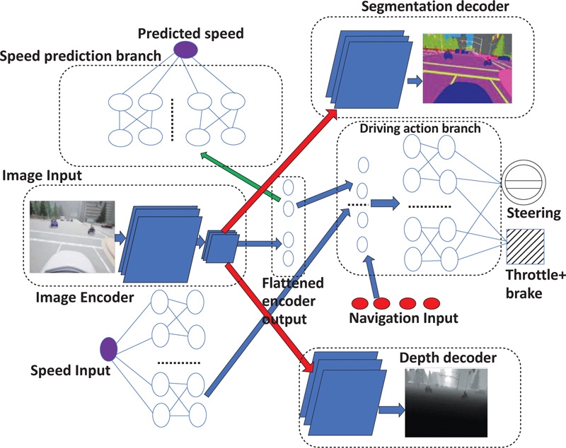
We use a modified version of U-Net [43] for image encoding and decoding for both image segmentation and depth mapping. Specifically, the encoder is implemented using MobileNetV2 [40] as a pre-trained encoder from Keras applications. The decoder is mainly derived using pix2pix [44] by up-sampling the encoder output, where implementation varies depending on the task, which will ultimately lead to one encoder and two decoders. To embed dynamic vision in the encoder, we predicted the speed of a vehicle using an RGB image. A high-level Neural network block diagram of the proposed CILDO model is given in Fig. (1).
As evident from Fig. (1), the output of the encoder is concatenated with an expanded dense layer from the speed measurement to obtain the perception for driving as the encoder is optimized for 3D static object detection by 2 decoders implemented for semantic feature detection, and depth vision and, at the same time, optimized for speed-related features from the speed prediction branch. Hence, all 3 types of perception required for autonomous driving, namely semantic features, depth and dynamic vision, will be completed. Therefore, the loss function (L) for the model will be composed of 4 terms, as shown in Equation 2.
 |
(2) |
 is the (i, j)th pixel value of the predicted segmentation image,
  is the (i, j)th pixel value of the ground truth segmentation image,
  is the (i, j)th pixel value of the predicted depth image, Pd (i,j) is the (i, j)th pixel value of the ground truth depth image,
  is the speed prediction, Mt is the ground truth speed,
  is the predicted action set, and At is the ground truth action set in Equation 2. Furthermore, in Equation 2, W is the total number of pixels in a line of the image across the width of the image, and H is the total number of pixels in one column of the image across the height of the image.
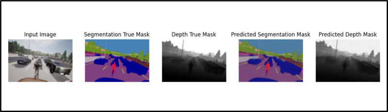
(Fig. 2) shows the input image, ground truth segmented image from a semantic camera, and ground truth depth image from a depth camera compared to the proposed CILDO model’s predicted segmented and depth images. The semantic segmentation camera converts a given pixel into one of 13 classes with corresponding color code, as given in Table 1 [45].
| Class | RGB Pixel Value | Color |
|---|---|---|
| Building | (70, 70, 70) |  |
| Other | (110,190,160) |  |
| Vegetation | (107,142, 35) |  |
| Poles | (153,153,153) |  |
| Traffic Lights | (250,170,30) |  |
| None | (70,130,180) |  |
| Road | (128,64,128) |  |
| Road Lines | (157,234,50) |  |
| Vehicles | (0,0,142) |  |
| Sidewalks | (244,35,232) |  |
| Fences | (150,100,100) |  |
| Walls | (145,170,100) |  |
| Pedestrian | (220,20,60) |  |
As observed from (Fig. 2), the model has been fairly able to predict the semantic and depth features simultaneously because only a small difference can be observed between the true masks and the corresponding predicted masks, as shown in Fig. (2).
2.1.2. Proposed Actor-Critic Model (CILDOLI-RL)
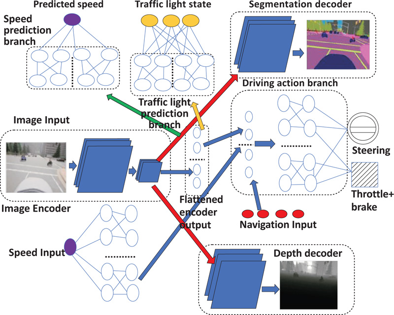
Compared to the CILDO model in Fig. (1), the CILDOLI-RL actor model has an additional loss function, and a neural network corresponding to the detection of traffic light state, as shown in the neural network, pointed out by the yellow-colored arrow in Fig. (3). We model the detection of 3-way traffic lights at a junction using the neural network to predict from the input image.
The additional branch corresponds to an additional loss function. Therefore, the loss function for the CILDOLI-RL model will be calculated using Equation 3.
 |
(3) |
TFt, TLt and TRt are the ground truth values of the forward lane traffic light state, left lane traffic light state, and right lane traffic light state, respectively, as given in Equation 3.  are the predicted values of the forward lane traffic light state, left lane traffic light state, and right lane traffic light state, respectively, as given in Equation 3. All other symbols in Equation 3 have the same meaning as for Equation 2.
2.1.2.1. Reinforcement Learning
Reinforcement learning allows an agent to learn how to behave in an environment. For the offline RL system, the environment is the simulated driving environment of CARLA, and the agent is the ego vehicle. However, due to the continuous nature of driving actions and states, initial exploration, as in the case of conventional reinforcement learning, can result in longer training times and a waste of resources. The initial exploration is drastically reduced by learning a base driving policy using imitation learning. A Markov Decision Process (MDP) in Reinforcement learning consists of environmental states (S = s1, ..., sN), actions (A = a1,…,aN), and transition function, which is a probability distribution between states T (s, a, s′) and a reward function for performing an action at a particular state to transit into a new state R(s, a, s′). The driving process can be considered an MDP since an action taken does not depend on previous observations and previous actions but only depends on the present observation [46]. The tuple (S, A, T, R) in MDP is called experience, and it should be stored in order to make decisions. The collection of such tuples stored over time is called an experience replay. The state and action spaces are not discrete but continuous variables in autonomous driving. The state S consists of an Image (I), the speed measurement (M) and control command (C) for autonomous driving using the CILDOLI-RL model.
For the proposed Actor-Critic, in particular, for reinforcement learning, we deviate from the batch reinforcement learning with experience replay [47] by only having a replay memory size of 2, storing only the present experience and previous experience.
2.1.2.2. Q-Learning
A state-action value function Qn(s, a) calculates how good it is to take action (a) in a given state (s) by following a policy π. It is defined as the expected return from future rewards, as shown in Equation 4 [48]:
 |
(4) |
In Equation 4, γ is called the discount rate, which is a positive constant less than 1, rt+k is the reward at (t+k)th time step, st is the state at time t, at is the action at time t, E is the expectation function, and Qπ(s, a) is the state-action value function obtained by following a policy Π.
The Q values need to be updated as rewards are obtained according to the Bellman Equation [46], as shown in Equation 5:
 |
(5) |
In equation 5, Qt(st, at) is the state-action Q value at tth time step for state at time t and action at time t, rt is the reward at (t)th time step, γ is the discount rate, max is the maximum function, which selects the maximum value from a given set of inputs, and α is the learning rate for updating Q values, which we set to 1 in this research to yield the following simplified equation, as shown in Equation 6.
 |
(6) |
In the proposed actor-critic model, the actor is the autonomous driving policy network (πa). The critic network is a value function, which is also a policy neural network (πc) having input as (S, A) and output as Q. Here, S and A are the state and action of the actor-network, respectively, and Q is the corresponding state-action value. The high-level neural network block diagram of the proposed CILDOLI-RL critic network is shown in Fig. (4).
Since autonomous driving involves continuous domain state-action pairs, the recently developed Deep Deterministic Policy Gradient (DDPG) algorithm is used to update the actor and critic’s model weights in reinforcement learning [49].

2.1.2.3. Deep Deterministic Policy Gradient (DDPG) Method
A deterministic policy (π: S |A) is a function belonging to the agent, mapping each state (S) input into an action (A). Therefore, the neural network that maps a given state to an action (CILDO) model is a Deep Deterministic Policy (DDP) network. The goal of reinforcement learning is to learn a policy called the optimal policy, which maximizes the rewards on a long-term basis. The DDPG method should update both the actor and critic network policies. Both actor and critic have 2 networks called the target model and the training model. Based on reinforcement learning using the rewards obtained per action, the training models of both the actor and critic are immediately updated, but the target models are updated at a selected learning rate (τ) by using weights from training models to converge target models to training models in the long run. The replay buffer consists of the present experience tuple and the previous experience tuple of the MDP. The DDPG process is as follows. Here, previous and current experience denotes two consecutive time steps (t and t+1) experience. The following set of actions is repeated for each new state-action pair.
- Reward rt for the previous predicted action is calculated using the reward function.
- For a given state (st+1), the target actor model predicts an action (at+1) using the target actor model’s policy (πaTar).
- Using the predicted action (at+1) and state (st+1), the target critic model predicts the Qt(st+1, at+1) value for the state-action pair using the target critic model’s policy (πcTar).
- Using the predicted action’s reward (rt), discount factor (γ), and predicted Qt(st+1, at+1) value from the previous step, using equation 6, updated Q value (Qt+1(st, at)), also called as the one-step return is found.
- From the replay buffer, the previous state (st) is selected. Using st, previous action (at) and training critic model’s policy (πcTra), Q value at tth time step for state at time t and action at time t (Qt(st, at)) is found.
- (Qt+1(st, at)) - (Qt(st, at)) is set up as the training critic model’s loss.
- The gradient of all trainable weights of the training critic network (DDP) with respect to the critic model’s loss computed in the previous step is calculated, and then weights are adjusted such that the critic’s loss is minimum.
- The gradient of all trainable weights of the actor-network (DDP) with respect to the Q value (Qt(st, at)) predicted by the training critic network called “critic value” is calculated, and then weights are adjusted such that the “critic value” is maximized.
- Finally, the target actor model and target critic models are updated at a learning rate of τ.
2.1.2.4. Reward Function
We closely associated our reward function with work done previously [37]. However, there were new components in our reward function, and changes were made to already existing components [37]. We defined the reward function (r), as given in Equation 7.
 |
(7) |
In Equation 7, rsteer is the reward for steering, rspeed is the reward for speed, rtraffic_light is the reward for moving in a traffic light, rdamage is the reward for collision damage, and roff_road is the reward for off-road driving.
In safe autonomous driving, the vehicle should obey the traffic lights. Therefore, we have introduced a reward for moving in a traffic light (rtraffic_light), as given in Equation 8:
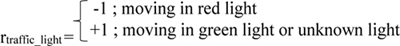 |
(8) |
The reward component for speed (rspeed) in a previous study [37] does not take into account the speed limits for the lane following function and provides a constant positive reward even at very high speeds. For the vehicle to follow the speed limits of the environment, we set the rspeed as shown in Equation 9:
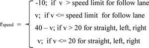 |
(9) |
Here, the speed limit is a variable whose value depends on the road on which a vehicle is driving, and v is the velocity of the vehicle.
Negative rewards are provided for steering (rsteer) in opposite directions for turning left or turning right or steering in either direction for going straight. The reward for collision damage (rdamage) is composed of negative rewards for collision with a vehicle, pedestrian, or any other object. The reward for off-road driving (roff_road) is composed of negative rewards for either moving in the opposite lane or crossing the sidewalk.
3. RESULTS AND DISCUSSION
CARLA is an open-source urban driving simulator used to develop, train and validate autonomous urban driving [2]. We used CARLA version 0.9.12 in our simulations. CARLA runs as a client-server system, which can be implemented in synchronous mode or asynchronous mode. We run all simulations in synchronous mode at a fixed frame rate of 8 FPS. The server waits until a clock tick is heard from the client, removing any possible error due to processing delays, such as prediction delays from neural networks.
3.1. Training Conditions
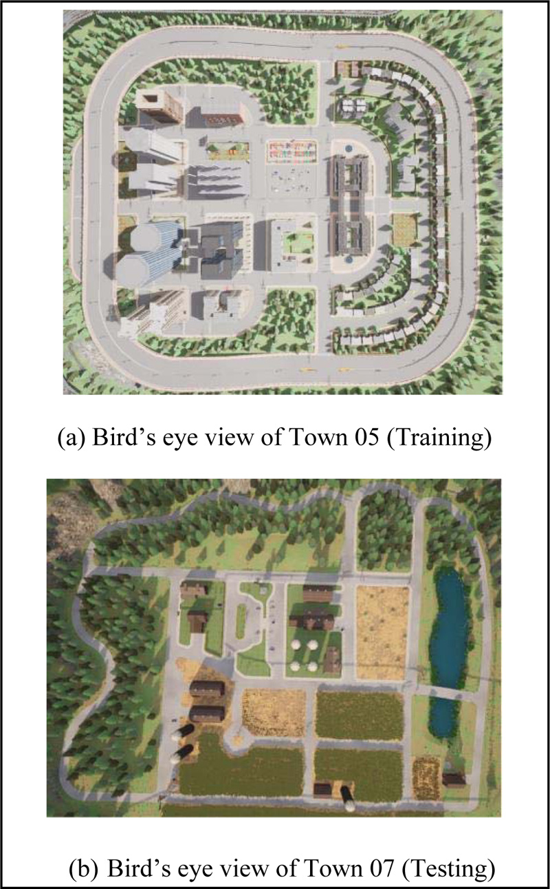
The camera poses fixed in space can lead to control errors and unexpected behaviors reinforcing each other [36, 50]. Therefore, we randomized the camera position from 0.10 to 0.25 times the length along positive X (length) direction and 1.5 to 2.0 times the height of the vehicle in Z (height) direction from the origin. We further randomized the camera pitch from 270 to 290 degrees, roll from 175 to 185 degrees, and yaw from -5 to +5 degrees. Here, the XYZ coordinate axes were a non-inertial frame of reference with origin at the centroid of the vehicle. In a real-world scenario, this will represent different fields of view of different drivers with different height and seat adjustments. This arrangement is more practical than a fixed first-person camera at the front of the ego vehicle, which always cannot see its parent vehicle [32]. Town 5 was selected as the training city, which was an urban town having multiple cross junctions and a bridge with multiple lanes per direction [51], as shown in Fig. (5a).
We set the weather randomly as dry or cloudy and change the lighting conditions randomly between {Noon, Sunset, and Night}. Afterward, we generated regular and dense traffic conditions for both the training and test conditions. The regular condition was 15 vehicles and 5 pedestrians per town, whereas the dense condition was 45 vehicles and 15 pedestrians per town. Training took place for all empty, regular, and dense traffic. In empty conditions, there were no pedestrians or other vehicles in the town except for the ego vehicle. We trained each model for any number of epochs until the predicted actions' loss was not decreasing. Neural networks were implemented using TensorFlow Version 2.6 and trained using the CPU version. The optimizer was selected as Adam with an initial learning rate of 0.0002, which decayed by 9% at the end of each epoch. The loss function is the mean squared error between the ground truth values and the predicted values. (Fig. 6) shows the training progress of each of the driving models which are trained in this context.
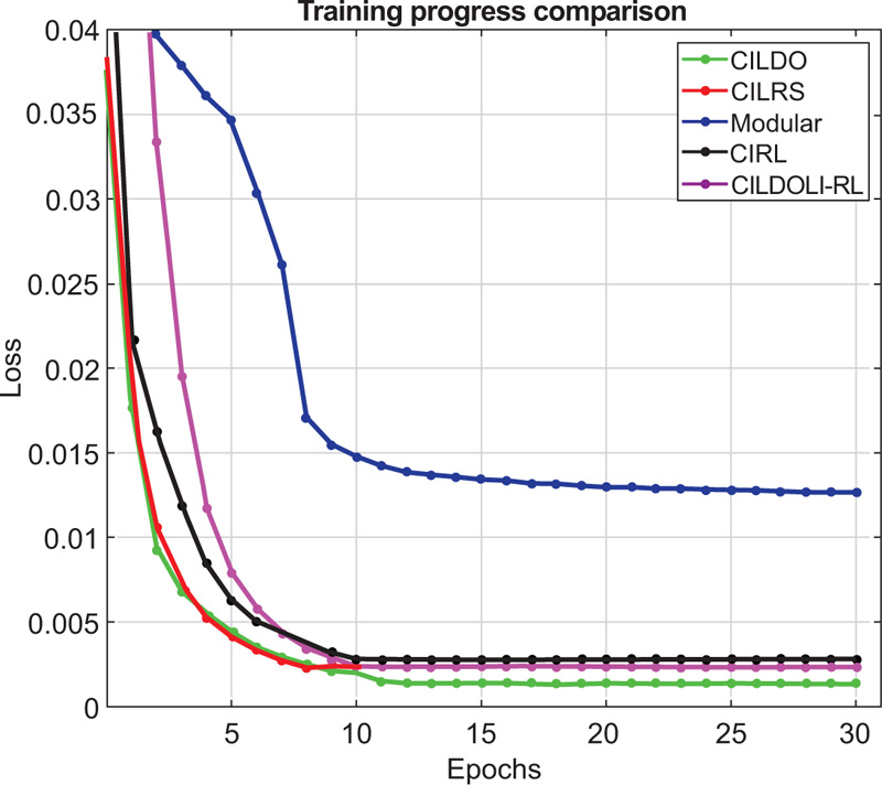
As evident from (Fig. 6), the modular approach has the highest loss out of the methods considered because, in the modular approach, the encoder is pre-trained separately before training the driving model. When the driving model is trained, the encoder’s training is frozen; therefore, its weights cannot be adjusted to minimize the predicted actions’ loss. On the other hand, the proposed CILDO method yields the least loss during training; therefore, higher driving performance can be expected from the CILDO method at the end of training for imitation learning.
The model at the end of each epoch is saved, and the model with the least loss is selected for testing. Since it has been found [32] that too much offline training on the data set can cause dataset bias in imitation learning, we trained all models compared in this work for a total of 8.9-hour-long demonstrations driven by an expert human driver for a fixed frame rate of 8 FPS, resulting a total of 256, 890 frames. Here, the navigation planning was also performed by the human driver and navigation instructions were also recorded. Due to the bottleneck in system memory during training, we resized the collected dataset to image frame resolution fixed at 120*80. For this data set, the human driver drove the vehicle following all road signs, traffic lights and road rules, unlike end-to-end driving [17]. The driving models can be tested for infractions, such as not following traffic lights, invading opposite lanes or sidewalks, and training for such data other than benchmarking for navigation and not crashing only. Therefore, we introduced a new benchmark for autonomous driving known as the No-Other-Infraction benchmark to further optimize driving and compare driving models. When we spawned the ego vehicle, we selected a random vehicle out of the vehicle blueprint library in CARLA from the 4-wheel category except for the class “Fire Truck”, which deviates by a large margin from the other vehicle categories in size and driver field of view. In particular, we picked a random vehicle of a random brand out of a random class, i.e., car, van, truck, SUV.
For reinforcement learning, we set the discount rate as γ = 0.99, learning rate in bellman equation α = 1.0, target model update learning rate (τ = 0.005), the critic’s learning rate of 0.001 and actor’s learning rate of 0.00001.
3.2. Testing Conditions
We fixed the camera position under testing conditions at 0 distance in the x-direction, 0.15 times height in the z-direction and pitch at 70 degrees to get the best field of view. An entirely different rural town, Town 7, as shown in Fig. (5b), is selected as a new town with only narrow roads and hardly any traffic lights [51]. Compared to town 5, town 7 had more y junctions, T-junctions, and turns that needed more steering with higher accuracy at a junction since the lanes were narrow. Therefore, driving is challenging in town 7. It should be noted that testing took place both in Town 5 and Town 7. When checking new weather, we set the weather randomly as wet or rainy with random changes in lighting as it was done for the training town, i.e., Town 5. Even though the training data set contained both day and night driving to provide data for feature detection under different lighting conditions, we tested both in town 5 and town 7 only in daylight to have consistent results. However, we kept a random selection of a driving vehicle as it was in training to represent a generalized driving model. TensorFlow CUDA-enabled GPU version was used to obtain predictions at a frame rate of 8 FPS. Out of all the possible spawn points for the vehicle from the Town, we selected a subset of spawn points by removing bad spawn points such as slopes, junctions, car parks etc. The ego vehicle was spawned at a random spawn point from the filtered subset in the corresponding town, and the vehicle should complete the intended navigation within 5 minutes to successfully complete an episode. The episode did not end at a collision, but all the collisions and other infractions (Not following traffic lights, driving in the opposite lane, sidewalk) were recorded to find the No-Crash benchmark and the new No-Other-Infraction benchmark introduced in this research.
| Training Conditions (Dry/Cloudy Urban Town) | Testing Conditions (Rainy Rural Town) | |||||||||
| Task | CILRS [32] | Modular [9] | CIRL [37] | Proposed CILDO | Proposed CILDOLI-RL | CILRS [32] | Modular [9] | CIRL [37] | Proposed CILDO | Proposed CILDOLI-RL |
| Straight | 91 | 60 | 92 | 94 | 86 | 89 | 70 | 90 | 94 | 80 |
| One Turn | 70 | 54 | 76 | 80 | 64 | 57 | 11 | 44 | 60 | 40 |
| Navigation | 60 | 36 | 55 | 70 | 60 | 25 | 8 | 25 | 30 | 20 |
| Dynamic | 51 | 14 | 49 | 62 | 46 | 13 | 4 | 13 | 21 | 11 |
| Task | CILRS [32] | CILDO without Depth Prediction | CILDO without Segmentation | Proposed CILDO |
|---|---|---|---|---|
| Straight | 89 | 91 | 90 | 94 |
| One-turn | 57 | 58 | 57 | 60 |
| Navigation | 25 | 28 | 27 | 30 |
| Dynamic | 13 | 20 | 15 | 21 |
3.3. CARLA Benchmark
The CARLA benchmark [2] benchmarks driving from simple going straight at the junction to navigation (Navigate with left and right turns at a junction) under dynamic objects in the training town and a new town with new weather. We selected training and test environments as specified in sections 3.1 and 3.2, respectively. CARLA benchmark is used to benchmark the navigation performance of driving models, where a high score for the benchmark indicates a high navigation performance. We compared the navigation performance of the proposed models with state-of-the-art driving models, as shown in Table 2, where we specified the number of times each of the navigation tasks was successful for 100 test runs. A high score for the CARLA benchmark indicates that the navigation performance of the particular driving models is high.
From the results in Table 2, it is crystal clear that the proposed CILDO method out-performs all other driving models for urban and rural navigation. The next highest performance for the training town is by CILRS, followed by the proposed CILDOLI-RL. The proposed CILDOLI-RL method sacrificed part of the navigation performance in order to obtain low other infractions, as evident from the following sections. For the urban town, the proposed CILDO method has significantly outperformed all other driving models. On the other hand, for the rural town with rainy weather, the proposed CILDO method slightly outperforms the CILRS model and significantly out-performs all other models in empty town conditions. This can be explained by the fact that the testing town is a rural town, and the semantic segmentation for the proposed methods has fewer classes to classify under no traffic conditions. However, when the rural town is concentrated with pedestrians and vehicles, the conditions become similar to urban with higher classes for semantic segmentation, so the proposed CILDO method significantly outperforms all other driving models. Therefore, the CILDO method has the generalization capability to perform in both urban and rural conditions. Furthermore, it is clear that reinforcement learning did not enhance navigation performance since the CARLA benchmark for CIRL or proposed CILDOLI-RL did not outperform other models entirely modeled from imitation learning.
In order to understand more about the performance gap between the proposed CILDO and CILRS in a rural town, we performed an ablation study, as explained in section 3.4.
3.4. Ablation Study
The ablation study was conducted to study the individual and overall effect of semantic segmentation and depth profiling on navigation performance. In the ablation study of the proposed CILDO model, the neural network and the loss function related to either semantic segmentation or depth detection were removed and trained. We obtained the results for the ablation study, where we reported the number of times the CARLA benchmark was successful per 100 test runs for each navigation task in town 7, as given in Table 3.
It is clear, according to the results in Table 3, that when the semantic segmentation is removed, the navigation performance reduces more than when the depth prediction is removed. Therefore, semantic segmentation has a higher impact on driving performance than depth prediction. Furthermore, when both are removed (conditions similar to CILRS), the combined effect is worse than when each of the semantic or depth predictions is removed, according to the results obtained in Table 3. Therefore, the proposed CILDO method is enhanced by semantic feature detection and depth prediction combined to give a higher navigation performance with a higher performance gap under dense traffic conditions than empty town conditions because, in the empty town, semantic segmentation has fewer classes to classify, hence its effect on navigation performance is lower than that for the dense town. This ablation study proves the reason for the increment of navigation performance in the proposed CILDO method.
3.5. No-Crash Benchmark
The No-Crash benchmark has been introduced previously [32], which considers an episode to be successful if there is no collision with another vehicle, pedestrian, or any other object. The No-Crash benchmark is used to test a driving model for the probability of collisions. Table 4 summarizes the percentage of No-Crash episodes for each of the driving models compared in this context, including the proposed 2 models per each 100 test runs in empty/regular/dense traffic conditions. A high score in the No-crash benchmark indicates that the particular driving model has less probability of collisions.
According to the results in Table 4, DDPG driven proposed CILDOLI-RL model out-performs all other driving models under an urban driving environment by a significant margin. In the rural town, for the case of regular and dense traffic, the proposed CILDOLI-RL model has the best No-Crash benchmark performance with a higher performance gap in dense traffic, as evident in Table 4. However, the performance gap is low for the No-Crash benchmark of the proposed CILDOLI-RL for the case of an empty rural town due to fewer classes for semantic object detection, as explained in the ablation study. On the other hand, the proposed CILDO model’s score for the No-Crash benchmark is moderate for the urban town and moderate for the rural town.
3.6. No-Other-Infraction Benchmark
We introduced the No-Other-Infraction benchmark by defining a successful event as if the vehicle does not drive off-road and follows all the road signs. Therefore, the No-Other-Infraction benchmark tests a given driving model for the probability of occurrence of other infractions, such as off-road driving and not following traffic signs except collisions. For the simulations of this paper, a road sign only refers to traffic lights and stop signs. However, in a real driving scenario, it refers to other road signs, such as speed limit signs, warning signs etc. So, if the No-Other-Infraction benchmark is successful, it means that the vehicle has not driven on the sidewalk or opposite lane, has stopped at all stop signs and obeyed traffic lights. This benchmark is important because the presence of a high score means the model has a lower potential for accidents. Table 5 summarizes the number of No-Other-Infraction episodes for each driving model compared in this context, including the proposed 2 models per each 100 test runs in empty/regular/dense traffic conditions. A high score in the No-Other Infraction benchmark indicates that there is a low probability of occurring other infractions.
It is evident from Table 5 that in an urban environment, the proposed CILDOLI-RL model out-performs all other models for the No-Other-Infraction benchmark by a large margin. This performance gap is due to the fact that none of the other models are trained or optimized to detect and obey traffic light state, while the CILDOLI-RL does both detecting by the imitation stage and conditioning to obey it by providing a positive reward at the reinforcement learning stage. The performance gap is lower in the rural town, which only has a few traffic lights and stop signs, unlike in town 5. In empty town 7, the performance gap between the proposed CILDOLI-RL and CIRL is very low. When the rural town is populated with vehicles and pedestrians, the performance gap between the CIRL and proposed CILDOLI-RL model increases with traffic density. It is due to the fact that the proposed CILDOLI-RL is favored by dense traffic conditions in terms of vision, as proved by the ablation study.
| Training Conditions (Dry/Cloudy Urban Town) | Testing Conditions (Rainy Rural Town) | |||||||||
| Task | CILRS [32] | Modular [9] | CIRL [37] | Proposed CILDO | Proposed CILDOLI-RL | CILRS [32] | Modular [9] | CIRL [37] | Proposed CILDO | Proposed CILDOLI-RL |
| Empty | 49 | 81 | 56 | 75 | 88 | 66 | 84 | 87 | 76 | 87 |
| Regular | 33 | 73 | 43 | 68 | 80 | 59 | 67 | 58 | 50 | 70 |
| Dense | 30 | 50 | 40 | 58 | 65 | 40 | 50 | 42 | 33 | 55 |
| Training Conditions (Dry/Cloudy Urban Town) | Testing Conditions (Rainy Rural Town) | |||||||||
| Task | CILRS [32] | Modular [9] | CIRL [37] | Proposed CILDO | Proposed CILDOLI-RL | CILRS [32] | Modular [9] | CIRL [37] | Proposed CILDO | Proposed CILDOLI-RL |
|---|---|---|---|---|---|---|---|---|---|---|
| Empty | 19 | 22 | 13 | 10 | 54 | 56 | 71 | 80 | 69 | 81 |
| Regular | 14 | 18 | 14 | 5 | 52 | 50 | 58 | 67 | 55 | 75 |
| Dense | 0 | 10 | 5 | 0 | 45 | 45 | 50 | 58 | 44 | 67 |
3.7. Inference Time
In autonomous driving, the prediction time of the driving model ultimately determines the rate at which actuators (throttle, brake, steering) can be driven. For high-speed driving, in order to achieve good driving performance, the prediction rate should be high. Therefore, when it comes to a driving model, not only its performance based on navigation capability (CARLA benchmark), collision-free driving (No-Crash benchmark), and no other infractions except collisions (No-Other-Infraction), but also the computational complexity of the model is important for testing at high speeds. We tested the driving model’s computational complexity using the average inference time for both CPU and GPU. The tested CPU was a 16-core Intel 11800H CPU running with Turbo Boost enabled, and the GPU was NVidia RTX3060. The result for average inference time in ms for each of the driving models is shown in Table 6. A low inference time for a given driving model indicates that the particular driving model is computationally efficient.
The modular pipeline approach for autonomous driving has the least average inference time, as evident from the results obtained in Table 6. Therefore, if the accuracy can be traded off for a higher frame rate at high speed, the modular pipeline will be the best model since it has the least computationally complexity for both CPU and GPU inference. On the other hand, proposed models are comparatively computationally less efficient and are more suitable for driving in dense urban environments with a moderate speed. This complexity occurs because of the additional decoder architecture for semantic segmentation and depth detection, and the proposed CILDOLI-RL model has an additional traffic light state prediction branch.
CONCLUSION
This paper proposed two driving models for fully autonomous driving. An ablation study proves that the three-dimensional dynamic object detection using image segmentation, depth prediction, and speed prediction in the imitation learning step improves navigation performance. The proposed CILDO model and the CILDOLI-RL have the highest and moderate scores for the CARLA benchmark, respectively, in both rural and urban towns. Regarding safety benchmarks, the proposed CILDO and the CILDOLI-RL models have moderate and the highest scores, respectively. Therefore, for safety-critical applications, such as for autonomous navigation of passenger vehicles in dense traffic driving scenarios, since both navigation performance and safety are crucial factors, it can be concluded that CILDOLI-RL is the best model out of the two proposed models. On the other hand, for applications that require navigation performance more than safety, such as humanless racing cars, agricultural robots etc., CILDO will be the most appropriate model. These findings will be valuable to optimize autonomous driving in diverse driving environments.
LIMITATIONS AND FUTURE WORK
Both of the proposed models are relatively computationally complex. The proposed models do not consider extended driving functions, such as reverse and forward parking functions at the end and beginning of navigation, lane changing and overtaking. These aspects need to be addressed in future work. Furthermore, the performance of the driving models with additional sensors, such as LIDAR, remains to be addressed.
AUTHOR CONTRIBUTIONS
P.A.D.S.N.W. contributed to conceptualization, methodology, software, validation, formal analysis, investigation, resources, data curation, writing–original draft preparation, review and editing, and visualization.
LIST OF ABBREVIATIONS
| CILDO | = Conditional Imitation Learning Dynamic Objects |
| CILDOLI-RL | = Conditional Imitation Learning Dynamic Objects Low Infractions-Reinforcement Learning |
| (MDP) | = Markov Decision Process |
| CAL | = Conditional Affordance Learning |
CONSENT FOR PUBLICATION
Not applicable.
AVAILABILITY OF DATA AND MATERIALS
The authors confirm that the data supporting the findings of this study are available within the manuscript.
FUNDING
None.
CONFLICT OF INTEREST
The author declares no conflicts of interest, financial or otherwise.
ACKNOWLEDGEMENTS
Declared none.

