All published articles of this journal are available on ScienceDirect.

Bridge Frost Prediction Using K-nearest Neighbor Classifier
Abstract
Background:
Considering the frequent occurrence of accidents on icy bridges during winter nights, it would be advantageous to notify both road managers and drivers regarding the most perilous areas. This notification would allow road managers to address the icy conditions by applying de-icing substances, while drivers could be more adequately prepared for potential hazards.
Methods:
In this study, the focus was on investigating k-nearest neighbor algorithms to predict nighttime icing caused by frost on three distinct bridges located on the National Highways in Korea. The algorithms utilized atmospheric data as input, which was obtained from the weather agency's website through an open API. The input data included relative humidity, air temperature, and dew point temperature, as well as the disparities in air temperature and humidity between two consecutive days.
Results:
In order to assess the effectiveness of the prediction models, reference data were created using the fundamental principle that ice is formed when the temperature of the pavement is below freezing and lower than the dew point temperature. Consequently, the developed algorithm demonstrated favorable performance, achieving an accuracy of 95% when evaluated using a test dataset that occupies 30% of the entire data.
Conclusion:
Considering the increasing focus on preventive maintenance, these newly developed forecasting models can be employed proactively as a preventive measure against icing. This proactive approach will ultimately contribute to improving traffic safety on winter roads.
1. INTRODUCTION
A significant number of traffic accidents occur on slippery roads. According to a study, these accidents lead to 1,300 fatalities and 13,735 injuries annually in the United States [1]. In Sweden, a report indicated that only 14% of drivers effectively adjust their speed on slippery surfaces [2]. Research conducted in Portugal suggests that the likelihood of a collision on icy roads is nine to ten times higher compared to dry surfaces [3]. In South Korea, data over a span of five years shows that 6,502 incidents on slippery roads resulted in 198 deaths. In 2019, a tragic accident took place on an icy bridge in South Korea, causing seven fatalities and numerous injuries. A similar incident occurred again in 2022.
Furthermore, the Korean government has instructed road maintenance agencies to incorporate pavement temperature measurements into their nighttime road maintenance patrols. These measurements serve as a foundation for implementing anti-icing initiatives [4]. Due to the fact that atmospheric sensors are typically situated far from the roads, reliable monitoring of road temperatures becomes challenging. Moreover, surface temperatures exhibit substantial fluctuations, even over short road sections, which restricts the practicality of using atmospheric temperature data for anti-icing purposes [5]. As a result, it becomes crucial to continuously measure pavement temperatures along the roadways to effectively combat black ice, particularly on bridges.
In general, snow removal operations are conducted according to weather forecasts, where snowplows are deployed to clear snow and apply chemicals either during or shortly before (1-3 hours) the snowfall. However, in Korea, the absence of black ice forecasts puts a significant strain on maintenance personnel. As a result, they are required to carry out daily patrols along the roads, imposing a substantial workload on them.
In order to address this problem, the present research focused on creating forecasting models for black ice to enhance the effectiveness of anti-icing operations, specifically targeting frost-induced black ice on bridges. A k-nearest neighbor model, a widely recognized machine learning algorithm, was employed, utilizing atmospheric data as input. By utilizing this forecasting model, nighttime occurrences of black ice can be predicted using daytime weather forecasts. This enables maintenance personnel to perform anti-icing activities, such as patrolling and applying chemicals only when the occurrence of black ice is anticipated.
2. LITERATURE REVIEW
Black ice can develop for several reasons [6], such as the overnight freezing of melted snow, the freezing of rain on the pavement with sub-zero temperatures, and frost bonding with the road surface. The first two causes can be anticipated through atmospheric weather forecasting since they are associated with snow or rain. However, the last cause can only be identified through routine road maintenance patrols [7].
In order to forecast black ice, traditional approaches have relied on physical models and regression analysis. Physical models utilize a surface energy balance model that considers heat conduction, convection, radiation, and vapor movement to estimate pavement temperature [8-11]. On the other hand, regression models predict pavement temperature using various data sources, including atmospheric data, geometric factors, and air temperature collected from probe cars [12-14]. However, both types of models have their limitations. Physical models require extensive data, such as pavement thickness, heat transfer rate of pavement materials, and heat flux, which may not always be readily available. This indicates that relying solely on atmospheric data and pavement temperature is insufficient for accurate black ice prediction. While easier to comprehend, regression models struggle with predicting variables that exhibit nonlinear correlations. Hence, this study employed a machine learning model to overcome the limitations of previous methods.
3. METHODOLOGY
The k-nearest neighbor (k-NN) algorithm is a versatile machine learning model employed for classification and regression tasks. It is categorized as a non-parametric algorithm since it does not assume any specific data distribution.
The functioning of the k-NN algorithm involves comparing a new data point to its k-nearest neighbors within the training dataset. The value of k is determined by the user. In classification tasks, the majority class label among the k-nearest neighbors is assigned to the new data point. In regression tasks, the predicted value is obtained by calculating the average or weighted average of the target values associated with the k-nearest neighbors.
The k-NN algorithm is straightforward and easy to understand, but its performance greatly depends on the choice of k and the distance metric utilized. Consequently, the quest for determining the optimal values of k and the distance metric becomes crucial in order to obtain a well-performing model.
4. RESULT
4.1. Data Collection
4.1.1. Pavement Temperature and Atmospheric Data
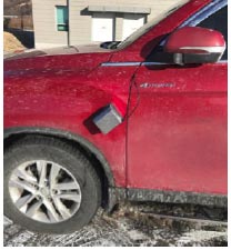
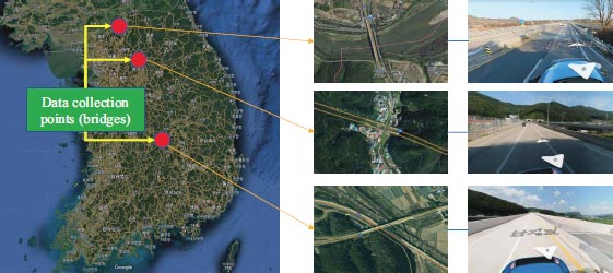
In this research, road maintenance vehicles were fitted with a road surface temperature sensor (depicted in Fig. 1), which utilizes an infrared thermometer to gauge the temperature of three bridges, as illustrated in Fig. (2). While the vehicle is in motion, the sensor is capable of measuring the temperature every 0.2 seconds. Pavement temperature data were obtained from three bridges, each approximately 300 meters in length, from December 2022 to February 2023. Data collection took place on a total of 397 days, with measurements recorded once per day during nighttime. Its precision is greatly enhanced by a narrow half-angle of 5°, resulting in accurate surface temperature measurements [15-17]. At 0°C, the sensor exhibits an accuracy of ±0.3°C. Furthermore, concurrent atmospheric data (air temperature and relative humidity) were acquired from the closest weather station during the same time period from an open API operated by the weather agency.
4.1.2. Pre-processing of Pavement Temperature Data
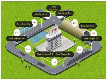
In order to efficiently utilize the gathered data for de-icing operations, it was crucial to consolidate the information according to specific roadway sections. To achieve this, the Korean government implemented a standardized node-link system (depicted in Fig. 3). This system divides the entire public highway network into nodes and links, taking into account various roadway characteristics, such as bridges, tunnels, overpasses, underpasses, intersections, and the number of lanes. Since the temperature of the pavement differs depending on the type of roadway, the aggregation of data using the node-link system is regarded as a logical and effective approach.
For the analysis of pavement temperature, the standard node-link system was employed to aggregate the data into a single median value on a daily basis, which served as a representative measure of central tendency. Nevertheless, as the measurements of pavement temperature obtained from moving vehicles may include outliers due to factors like debris on the road, driving on the shoulder lane, intermittent stops during patrolling, and so on, it was crucial to adopt a careful aggregation method to address any unforeseen consequences caused by these outliers. Among the three commonly used measures of central tendency (mean, median, and mode), the median was chosen because it is less influenced by extreme observations [18, 19].
4.1.3. Analysis of Pavement Temperature and Atmospheric Data
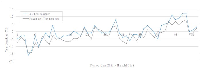
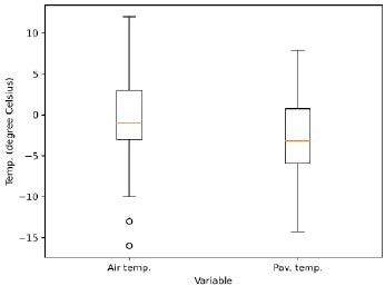
Fig. (4) depicts a graph illustrating the pavement temperature and air temperature recorded at one of the aforementioned three bridges. Similar patterns were observed at the other two bridges. Overall, the bridge temperature was consistently lower than the air temperature, with the air temperature exhibiting greater variability. table 1 and 2 display that, on average, the bridge temperature was approximately 2 times lower than the air temperature, while the maximum temperature reached about 4 °C higher. In contrast, the air temperature had a minimum temperature of approximately 2 °C lower than the pavement temperature. Unlike the air temperature, which fluctuates considerably due to air flow, the pavement temperature is presumed to exhibit relatively low variability due to the geothermal and latent heat properties of the structure, as shown in Fig. (5).
| Statistics | Air Temp. | Pav. (Bridge) Temp. |
|---|---|---|
| Mean | -0.30 | -2.47 |
| Standard deviation | 5.56 | 5.01 |
| Minimum | -16.00 | -14.30 |
| 25% | -3.00 | -5.93 |
| 50% | -1.00 | -3.15 |
| 75% | 3.00 | 0.73 |
| Maximum | 12.00 | 7.90 |
| Index | Score |
|---|---|
| Accuracy | 0.95 |
| Precision | 0.97 |
| Recall | 0.93 |
| F1 score | 0.95 |
4.2. Bridge Frost Prediction
4.2.1. Building Blocks of K-Nearest Neighbor Models
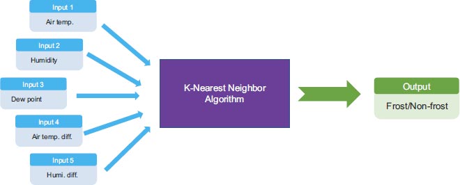
A predictive model for nighttime black ice using atmospheric data was established. The input data for a k-NN model included temperature, humidity, dew point temperature, temperature differences between consecutive days, and humidity differences between consecutive days (see Fig. 6). These data were collected over a span of two years at the three bridges mentioned earlier. To create the baseline data, we combined the input data with pavement temperature data obtained from patrol vehicles. Detailed information regarding the baseline data will be presented in the subsequent chapter. The configuration of the k-NN model is illustrated in Fig. (6). Since the scales of the input data varied, we applied standard scaling to normalize the data prior to training the models. The training and test sets were divided into a 7:3 ratio, and the raw data were classified based on the ratio of dry/icing conditions to ensure a balanced distribution in both sets. The analysis encompassed a total of 397 days, with 193 days classified as icy conditions and 204 days as dry conditions.
4.2.2. k-NN Algorithm Procedure
To implement the k-NN algorithm in Python, the following steps were followed:
1. Load the labeled training dataset, which contains input feature vectors and their corresponding class labels or target values.
2. Choose a value for k, which represents the number of nearest neighbors to consider during predictions.
3. Compute the distances between a new input sample and all the training samples using a distance metric. This metric quantifies the similarity or dissimilarity between two data points.
4. Identify the k-training samples with the smallest distances to the input sample. These samples will be the nearest neighbors.
5. For classification tasks, assign the class label that appears most frequently among the k-nearest neighbors to the input sample.
4.2.3. Finding Optimal Parameters
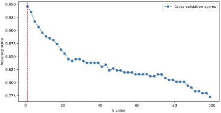
Finding the best value for k is crucial in the k-nearest neighbors (k-NN) algorithm. A small k can lead to overfitting, making the model overly sensitive to noisy data. Conversely, a large k can result in over-smoothing, causing the model to overlook local patterns in the data. The optimal value for k is typically determined through techniques like cross-validation or grid search. These methods involve evaluating different k values and selecting the one that performs best based on evaluation metrics. Fig. (7) illustrates the process of selecting the optimal k value, with a value of one being identified as the optimal choice.
4.2.4. Optimal Metric Selection
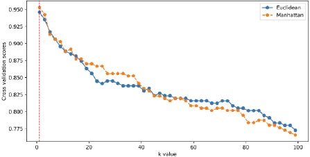
The choice of distance metric in the k-nearest neighbors (k-NN) algorithm depends on the characteristics of the data and the specific problem being addressed. Euclidean and Manhattan distances (Eqs. 1 and 2) are commonly used options. Therefore, the selection of the optimal metric was performed for these two metrics, as shown in Fig. (8). The analysis revealed that for a value of k equal to one, the optimal metric was found to be the Euclidean distance. Typically, k-NN algorithms can be computationally expensive when dealing with large datasets, as they involve calculating distances for each new sample against all the training samples. However, in this study, the data size was relatively small (only a few bytes), which did not pose a hindrance to the extensive computations.
 |
(1) |
 |
(2) |
where d(x,y) = distance between points x and y.
4.3. Assessment
4.3.1. Baseline Data Generation
To assess the precision of the predicted black ice data, it is crucial to establish a baseline. While employing a reference device to directly measure the road surface conditions would be the most reliable and straightforward approach, it was not feasible within the scope of this study due to labor-intensive requirements, costs, and the need for device acquisition. Instead, we relied on a physical principle described in Eq. (3), which indicates that frost develops on the pavement when the pavement temperature is not only below freezing but also lower than the dew point temperature.
 |
(3) |
where Tp = pavement temperature and Td = dew point temperature.
The concept of dew point temperature pertains to the specific temperature at which moisture in the air reaches saturation, resulting in the formation of fog or frost and causing the relative humidity to reach 100%. To determine the dew point temperature, the commonly employed approach is to utilize the Magnus formula, which is a widely accepted method for this purpose [15]. This formula calculates the saturation vapor pressure over liquid water at a given temperature (T) using Eq. (4).
 |
(4) |
The Eq. (4) incorporates the parameters α (6.112 hPa), β (17.62), and λ (243.12°C). By rearranging the terms in Eq. (4), we can derive Eq. (5), which provides an expression for the dew point (Td) based on the vapor pressure.
 |
(5) |
By substituting the definition of relative humidity (E=RH*EW/100) into Eq. (5), we can derive Eq. (6), which enables us to calculate the dew point (Td) using both the atmospheric temperature (T) and relative humidity (RH).
 |
(6) |
Eqs. (4-6) employ the well-established Magnus formula, which is widely recognized as a reliable method for estimating the dew point temperature using the atmospheric temperature and relative humidity. This formula exhibits an error rate of approximately 0.35°C [16].
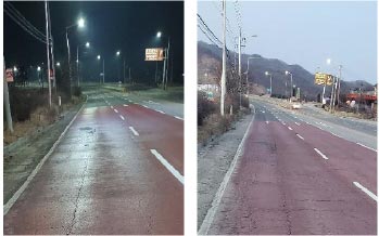
To validate the precision of the Magnus formula, a winter road segment was surveyed, specifically focusing on frost-induced black ice occurrences. It was observed that black ice formed (on the left) when the criteria for frost formation were satisfied, whereas no black ice was observed (on the right) when those criteria were not met, as depicted in Fig. (9).
| Classification | Prediction | ||
|---|---|---|---|
| Dry | Icy | ||
| Baseline | Dry | 0.935 | 0.065 |
| Icy | 0.034 | 0.966 | |
4.3.2. Performance of k-NN Model
The developed model was evaluated using a test dataset consisting of 119 samples, which accounted for 30% of the entire data, and the performance is presented in Table 1. The evaluation metrics used, including accuracy, precision, recall, and F1 score, are commonly employed to assess the effectiveness of machine learning models. These metrics, as defined in Eqs. (7-10), indicate that the model yielded satisfactory outcomes with accuracy, precision, recall, and F1 score values of 0.95, 0.97, 0.93, and 0.95, respectively. Additionally, Table 3 showcases the confusion matrix, which further demonstrates the model's strong performance across all cases. Particularly noteworthy is its capability to accurately identify “icy” conditions, which is crucial for winter road maintenance.
 |
(7) |
 |
(8) |
 |
(9) |
 |
(10) |
5. DISCUSSION
Conventionally, the Road Weather Information System (RWIS) has been used to predict black ice. To utilize RWIS, Environmental Sensor Stations (ESSs) are essentially deployed on the road, implying a substantial budget need to be allocated. Unfortunately, no available RWIS ESSs are installed in Korea. In this regard, predicting frost-induced nighttime black ice using readily available atmospheric data can be regarded as a cost-efficient countermeasure. Additionally, weather phenomena are known to be recurrent, indicating that the k-NN model developed in this study could be effectively applied. The suggested model can be practically applied to nighttime road maintenance patrolling, which would make winter road maintenance resources more efficient.
It should also be noted that the baseline data employed in this analysis do not directly reflect the actual surface conditions observed in the field. Instead, these values are calculated using road surface temperature and atmospheric data. Additionally, it should be noted that even when the conditions for frost formation are met based on physical laws, road icing may not occur in situations with high traffic volume [20, 21]. Nonetheless, the findings of this study hold significant value from various perspectives. From the standpoint of road administrators, if the presence of icing due to frost is anticipated, they can proactively engage in anti-icing measures. In this regard, the outcomes of this study can be practically applied to real-world winter road maintenance activities.
CONCLUSION AND FUTURE STUDIES
In Korea, the occurrence of accidents caused by black ice, which led to seven fatalities in 2019 and numerous injuries in 2023, has prompted significant changes in winter road maintenance practices. As a response, field workers have been assigned daily maintenance patrols throughout the winter season. However, there has been a growing demand among field personnel for an improved patrolling schedule, particularly concerning the development of nighttime ice predictions.
Currently, there are no available predictive models specifically for bridge frost treatment using atmospheric data. As a result, maintenance patrols are often conducted on bridges even when the occurrence of black ice is not anticipated, leading to inefficiencies in terms of labor and equipment. To address this issue, a reliable machine learning model using k-NN was explored to predict the potential for nighttime black ice, yielding satisfactory results with an accuracy rate of 95%. Notably, the strength of this model lies in its ability to forecast bridge frost solely based on atmospheric data, making it highly applicable to real-world scenarios. Utilizing the findings of this study, winter road maintenance personnel can streamline their patrols by focusing solely on predicted occurrences of black ice. This approach makes winter road patrol activities more efficient and scientifically informed.
However, it is essential to note that the evaluation of the k-NN model was solely based on baseline data derived from a physical principle. In the future, if feasible, it is recommended to gather baseline data through field observations using a device that accurately measures road slipperiness to ensure a more robust evaluation process.
LIST OF ABBREVIATIONS
| k-NN | = k-Nearest Neighbor |
| RWIS | = Road Weather Information System |
| ESSs | = Environmental Sensor Stations |
CONSENT FOR PUBLICATION
Not applicable.
AVAILABILITY OF DATA AND MATERIALS
The data and supportive information are available within the article.
FUNDING
This work was financially supported by a grant (No. KMI 2002-00110) from the Korea Meteorological Institute (KMI).
CONFLICT OF INTEREST
The author declares no conflict of interest, financial or otherwise.
ACKNOWLEDGEMENTS
Declared none.

