All published articles of this journal are available on ScienceDirect.

Effect of Night-time Rainfall on Traffic Stream Deterioration of Roads without Light
Abstract
Background:
This paper fills an important gap in the on-going road lighting debate by investigating traffic stream deterioration during night-time rainfall.
Introduction:
The study carried out an investigation into the impact of night-time rainfall on traffic stream deterioration of two-lane roadways without.
Methodology:
In the rainfall impact studies, traffic volume, speed, vehicle type and headway data were collected at selected road segments in Akure, Nigeria. All surveyed roadways were within rain gauge catchment area of about 1km. Rainfall intensity was divided into three groups (light, moderate, and heavy). Dry weather data were used as a control parameter.
Data Analysis:
Stepwise data analysis is used for the ease of explanation and clarity. All model equations were tested for statistical fitness and deemed satisfactory for further analysis.
Results:
From the result, it is observed that rainfall intensity influences traffic flow at night-time.
Conclusion:
Based on the results and findings, it is correct to conclude that the effect of night-time rainfall on traffic stream deterioration of roadways without lighting is significant. It is also correct to assert that rainfall affects night-time traffic stream performance on roads without lighting.
1. INTRODUCTION
Nigeria is faced with the problem of insufficient electricity supply to the extent that roadways are without road lights. Driving on such a road at night is challenging as a result of impaired visibility. Nigeria is still saddled with poor provision of road system that often, dark roads are traffic stream optimization constraints at night. Nigeria roads are classified as: Trunk A federal, Trunk B state and Trunk C local with majority of the roads in poor conditions. Given that the roads promote social development and foster economic growth, the tests of optimising traffic stream characteristics would call for roads irrespective of classification to have functional lights and the road surface. According to the report of Ayeni & Oni (2012) and Nzoiwu et al. (2017) [1, 2], road accidents increase during the wet season in Nigeria, therefore, it may be correct to assume that roadways without light may be death traps at night when it rains. Generally, it has been shown in previous studies that driving under rainy conditions has an impact on traffic flow, speed, travel time and capacity. However, previous studies focused on roads with lighting considered rainfall occurrences as a source of uncertainty capable of affecting traffic regarding safety and operation [3-5]. Note that previous studies were on road traffic under rainy and daylight conditions. The quantitative measure which describes the traffic carrying ability of a road facility is the capacity. It plays an indispensable part in evaluating traffic performance. Highway Capacity Manual (HCM), 2010 [6] defined capacity as the maximum hourly flow rate by which vehicles or persons are expected to pass a certain point or uniform section of a roadway for a certain period of specific roadway, traffic, geometric, control and environmental conditions. In this paper, uninterrupted traffic flow, speed, density and capacity reduction triggered by night time rainfall on roads without lighting have been investigated. Generally, traffic streams are not uniform, but vary over time and space. Consequently, measurement of their variables is in fact the sampling of a random variable. It is postulated that night time travel stream characteristics on roadways without light are likely to change and induce capacity loss during rainy conditions.
2. BACKGROUND
Estimation of road capacity has received considerable attention in the past studies. Past studies have tried to estimate capacity using different methods but arrived at different values. Most of the studies relied on the theory of traffic flow using traffic flow, speed, density and headway. Minderhoud et al. [7] reported that capacity using empirical data could be estimated by the following methods viz headways, estimation using traffic flow (selected maxima method, expected extreme value and bi-modal distribution method), use of traffic flow and speed (Product Limit method) and use of traffic flow, speed and density (fundamental diagram). Usage of each method depends on various conditions which include location choice for observation, required observation period, type of data to be collected, lane or carriageway and traffic state. Headway and fundamental diagrams estimation method are used for off-peak traffic state. Since the interest of this study is at night-time which is off peak travel, flow/density modeling technique is adopted in this paper. Flow/Density function relies on the fundamental relationship of flow, speed and density. According to Ben-Edigbe (2010) [8], use of fundamental diagram for capacity estimation is good, based on the following advantages. Firstly, the fundamental diagram does not require getting data at a bottleneck for capacity to be estimated, therefore traffic state can be determined at any point. Secondly, with two known variables, the other variable could be determined. Lastly, the flow/density method could be used to model different conditions of traffic. Studies that had used fundamental diagram to study traffic conditions include Billot (2009), Lam et al., (2013), Ben-Edigbe et al. (2014), Hassan et al. (2016) [9-12]. The general equation for the flow-density relationship is given as:
 |
(1) |
Where; q – flow, k – density, uf - free flow speed, and kj - jam.
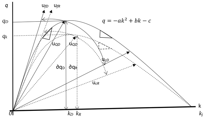
According to Greenshields (1935) [13], the symmetry curve shows that the rate at which density increases is the same for the uncongested and congested sections of the curve. This may not be true as it could be argued that the symmetric curve does not give a true representation of traffic stream characteristics. According to Ben-Edigbe (2014) [8], traffic breakdowns occur when traffic becomes unstable and exceeds 40 vehicles per lane-km. According to Knoop and Daamen (2017) [14], “Jam density” refers to extreme traffic density when traffic flow stops completely, usually in the range of 185–250 vehicles per mile per lane (120-160 vehicles per lane-km). Ben-Edigbe (2014) [11] argued that one kilometre of road is fixed and would take a finite number relative to the type and percentage of the vehicles. For example, 1km road length with passenger car concentration of 5.5m per vehicle would yield about 180 vehicles at jam density. The asymmetric curve is based on the premise that traffic behaviour in the unconstrained section is not the same as that of the constrained section. For other countries like USA and Japan with 6.5meter and 5.0meter occupancy respectively, their jam densities are 154veh/km and 200veh/km. As shown below in Fig. (1), traffic stream characteristics and capacity are expected to shift as a result of the prevailing condition. According to Fig. (1), O AD B represents the path of traffic operation under normal and dry conditions. At point O, the initial stage of traffic flow, density and flow are zero but as flow increases, density will also increase along path OB. When traffic flow reaches point AD, it is said to be at its maximum and it is represented as qD=qm while its corresponding density is at kD. Further, increase in the number of vehicles will follow path AD B with a corresponding increase in density till it reaches kj. At this point, speed will become zero and traffic is said to be in jam state (congested condition). Alternatively, under rainy conditions, traffic operation is assumed to follow path O AR B as shown in Fig. (1). The maximum flow under rainy condition is given as qR with corresponding density kR and speed at capacity UQ R. From the above, there is a shift in the traffic operation path with corresponding changes in subsequent traffic flow parameters as depicted in the figure. Thus, it is postulated that;
Free flow will shift from ufD to ufR; Speed at capacity will shift from uQD to.
Congestion speed will shift from ucD to ucR; Traffic flow will shift from qD to qR
Traffic Density will shift from kD to,
 |
(2) |
 |
(3) |
Where; q – flow, k – density, u – speed; R – rain; D – .
Xu et al. (2013) [5] considered rainfall occurrences as a source of uncertainty capable of affecting traffic in terms of safety and operation. Mukhlas et al. (2016) [15] stated that increase in rainfall intensity leads to speed and capacity reduction. In a study carried out by Alhassan and Ben-Edigbe (2012) [16], capacity loss of 1.08%, 6.27% and 29.25% was reported for light, moderate and heavy rain, respectively. Capacity by its definition is stochastic, meaning it has no set value. The capacity estimation method by Minderhoud (1997)
[7] was modified by Brilon (2005) [17] based on the earlier works of Kaplan and Meier (1959) [18] product limit method and van Toorenburg (1986) [19] distribution function. The modified method is written as:
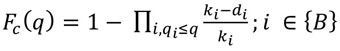 |
(4) |
where; Fc (q) = distribution function of capacity c
q = traffic volume veh/h
qi = traffic volume in interval i veh/h
ki = number of intervals with a traffic volume of q ≥ qi
di = number of breakdowns at a volume of qi
{B} = set of breakdown intervals
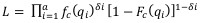
Note that complete distribution function is only possible if maximum observed volume is followed by breakdown and recovery. Otherwise, it would be impossible to reach a complete distribution function as the function will terminate in a value less than one. Accordingly, a complete capacity distribution function is rarely reached; even if reached, it might not be so reliable in higher volumes, unless a huge size of data is gathered. Product limit method on the other hand does not require the assumption of a specific type of distribution function according to Brilon (2005) [19]. Maximum likelihood estimation is a method that determines values for the parameters of a model. The parameter values are found such that they maximise the likelihood that the process described by the model produced the data that were actually observed. Clearly, by its name, the maximum likelihood method is a parametric technique, and its success depends on the validity of the distributional assumptions made. In order to estimate the parameters of the distribution functions, a maximum likelihood technique is given by Lawless (2003) [20] as;
 |
(5) |
Where; fc (qi) = statistical density function of capacity c
Fc (qi) = cumulative distribution function of capacity c
n = number of intervals
δI = 1, if uncensored (breakdown of classification B)
δI = 0, elsewhere
Transformed into capacity analysis, Log-likelihood function is rewritten as:
 |
(6) |
3. MATERIALS AND METHODOLOGY
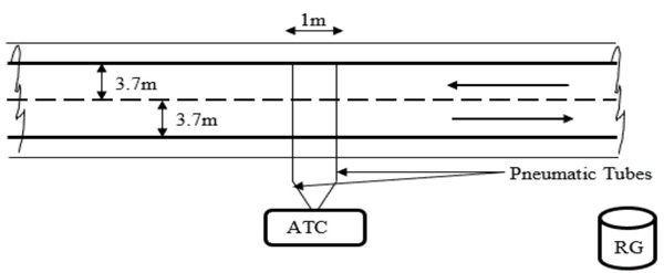
Traffic and rainfall data were collected continuously for eight weeks at four selected two-lane highway without road light in Nigeria. Proximity to rain gauge catchment range was sacrosanct to the study. Selected sites were straight with flat terrain with functional drainage system and free from pavement distress. Traffic data were collected with an Automatic Traffic Counter (ATC) as shown below in Fig. (2). It is important that the segment Length (L) be greater than sight distance (SSD) in order to increase the probability of unbiased vehicle data collection. As shown in Fig. (2), two sensor tubes set at one meter apart were attached to the ATC counting machine. Vehicle information captured by the ATC included the following: speed, volume, weight, headway, gap, type of vehicle, date and time of vehicle hit. Note that RG denotes rain gauge. It is important that the survey site must lie wholly within the catchment area of the rain gauge.
The main study was carried out in Akure, Nigeria whilst pilot study was done in Durban, South Africa. Over 500,000 vehicles were recorded. Rainfall data were obtained using rain gauge with data-logger. The data-logger records rainfall events at 1-minute interval continuously. Using a 5-min interval, the obtained data was separated into daylight and night-time data. The rainfall precipitation amount was converted into intensity and separated into light (i < 2.5mm/hr), moderate (2.5 ≤ i < 10 mm/hr), heavy (10 ≤ i < 50 mm/hr) and very heavy (i > 50mm/hr) rainfall in line with World Meteorological Organisation classification.Very heavy rainfall was not considered in the study.
4. RESULTS AND DISCUSSION
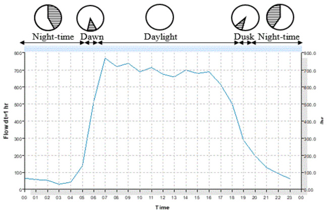
Traffic data was separated into daylight and nigh time. Traffic data between 7.30pm - 11pm was considered for night-time as traffic flows beyond 11pm are usually characterised by heavy vehicles, high headways and low volume. As shown below in Fig. (3), typical 24hr traffic flow activities on roads without light in Nigeria are time dependent. Traffic flow activities pick up around 6 A.M and gradually slow down around 6 P.M. Traffic flow within the period of 7.30 pm - 11 pm was considered for night time. Traffic flows beyond 11 pm are usually low (below 100veh/h) and characterised by high headway and heavy good vehicles. Stepwise analytical method was adopted for clarity and procedural ease.
Step 1: Use modified passenger car equivalent values to convert traffic volume to flow. Separate and group traffic data into daylight / night time; dry / rainfall. Separate and group rainfall data into light, moderate and heavy as shown below in Table 1. Compute density (k) from flow (q) and speed (u) data. For example, when speed u = 70km/hr and flow q = 210pce/h, then density k = 210/70 = 3pce/km.
| Dry Night-time | Rainfall Intensity at Night on Roadway without Light | ||||||||||
|---|---|---|---|---|---|---|---|---|---|---|---|
| Light Rain i≤2.5mm/h | Moderate Rain i≤10mm/h | Heavy Rain i≤50mm/h | |||||||||
| u | q | k | u | q | k | u | q | k | u | q | k |
| 70 | 210 | 3.0 | 49 | 195 | 4.0 | 57 | 240 | 4.2 | 62 | 255 | 4.1 |
| 81 | 300 | 3.7 | 65 | 375 | 5.8 | 50 | 143 | 2.9 | 52 | 263 | 5.0 |
| 80 | 300 | 3.8 | 45 | 240 | 5.4 | 62 | 210 | 3.4 | 65 | 165 | 2.5 |
| 70 | 195 | 2.8 | 65 | 165 | 2.5 | 70 | 240 | 3.4 | 47 | 60 | 1.3 |
| 87 | 180 | 2.1 | 68 | 248 | 3.7 | 65 | 180 | 2.8 | 74 | 135 | 1.8 |
| 62 | 195 | 3.1 | 73 | 210 | 2.9 | 76 | 150 | 2.0 | 49 | 233 | 4.7 |
| 85 | 450 | 5.3 | 61 | 173 | 2.8 | 63 | 90 | 1.4 | 56 | 180 | 3.2 |
| 75 | 323 | 4.3 | 60 | 480 | 8.0 | 50 | 135 | 2.7 | 53 | 158 | 3.0 |
| 66 | 195 | 3.0 | 70 | 203 | 2.9 | 64 | 150 | 2.3 | 40 | 90 | 2.3 |
| 60 | 293 | 4.9 | 68 | 383 | 5.6 | 60 | 150 | 2.5 | 82 | 188 | 2.3 |
| 75 | 248 | 3.3 | 52 | 120 | 2.3 | 75 | 150 | 2.0 | 55 | 195 | 3.5 |
| 81 | 248 | 3.1 | 57 | 300 | 5.3 | 55 | 120 | 2.2 | 62 | 225 | 3.6 |
| u | q | k | PC% | LGV% | HGV% | kj-pc | kj-LGV | kj-HGV | kj-total |
|---|---|---|---|---|---|---|---|---|---|
| 70 | 210 | 3 | 95 | 4 | 1 | 172.7 | 6.2 | 1.3 | 180 |
| 81 | 300 | 3.7 | 87 | 10 | 3 | 158.2 | 15.4 | 3.8 | 177 |
| 80 | 300 | 3.8 | 88 | 8 | 2 | 160.0 | 12.3 | 2.5 | 175 |
| 70 | 195 | 2.8 | 90 | 9 | 1 | 163.6 | 13.9 | 1.3 | 179 |
| 87 | 180 | 2.1 | 92 | 7 | 1 | 167.3 | 10.8 | 1.3 | 179 |
| 62 | 195 | 3.1 | 98 | 1 | 1 | 178.2 | 1.5 | 1.3 | 181 |
| 85 | 450 | 5.3 | 90 | 7 | 3 | 163.6 | 10.8 | 3.8 | 178 |
| 75 | 323 | 4.3 | 91 | 8 | 1 | 165.5 | 12.3 | 1.3 | 179 |
| 66 | 195 | 3 | 90 | 7 | 3 | 163.6 | 10.8 | 3.8 | 178 |
| 60 | 293 | 4.9 | 89 | 9 | 2 | 161.8 | 13.9 | 2.5 | 178 |
| 75 | 248 | 3.3 | 90 | 8 | 2 | 163.6 | 12.3 | 2.5 | 178 |
| 81 | 248 | 3.1 | 91 | 7 | 2 | 165.5 | 10.8 | 2.5 | 179 |
| - | - | Total | 1091 | 85 | 22 | 1983.6 | 130.8 | 27.5 | 2142 |
| - | - | Average | 91 | 7 | 2 | 165.3 | 10.9 | 2.3 | 178 |
Step 2: It was postulated that asymmetrical curve would be used in the paper.Table 2, jam density is a function of vehicle composition, type and concentration per kilometre per lane. Using 5.5m for passenger car, 6.5m and 8m for light (LGV) and Heavy Good Vehicles (HGV) respectively for vehicle type occupancy on road, hence,
jam density, kj = kj-PC + kj-LGV + kj-HGV;
where Passenger cars, kj-PC = {(col 4 /100) *(1000/5.5)}
Light good vehicles, kj-LGV = {(col 5/100) *(1000/6.5)}
Heavy good vehicles, kj-HGV = {(col 6/100) *(1000/8)}
Step 3: Determine flow/density model equations for all scenarios and test for statistical fitness as illustrated below in Fig. (4). The models have coefficient of determination r2 greater than 0.5 which signifies that the variables are significant.
Step 4: Using the derived model equation in step 3 above to determine density at capacity (kQ), traffic capacity (Q) and speed at capacity (uQ). For example, using model equation of dry night-time condition given as equation 7
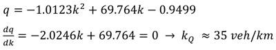 |
(7) |
Traffic capacity Q is estimated from equation 4 as
Q = -1.0123 * (35)2 + 69.764 * (35) - 0.9 Q = 1201 Pcs/hrSpeed at capacity 
Free flow speed from equation 4 ≈ 70km/h (69.764)
For jam density = 178veh/km; Hence congested density = 178 – 35 = 143veh/km
Congestion speed = 1201/143 = 8km/h
Step 5: Construct the flow, speed density asymmetric curve with the information in step 3 (Fig. (5) below) and
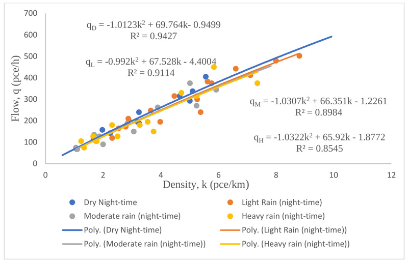
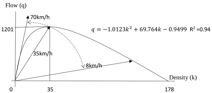
show that free flow speed will decrease gradually from 70km/h to 35km/h at traffic capacity and the congested section of the curve. It will decrease further to 8km/h as it tends to zero. It confirms the assertion expressed by Mukhas et al. (2016) [15]. The procedure is repeated for all sites and all scenarios.
It is apparent from the investigations so far that the effectiveness of road use has been constrained by darkness and rainfall among others. The shift from left to right in flow / density curve as shown in Fig. (5) is indicative of constraint on the roadway. The shape of the flow / density curves for all locations indicated that flow first rises and later falls as density rises from zero to critical. When the traffic operates at capacity, further increase in density will not result into increase in flow.
Step 6: Estimate rainfall impact on roads without lighting traffic characteristics. As shown below in Table 3, the free flow traffic stream characteristics are flow, speed, density, headway and spacing. Note that spacing (s) = speed x headway. Results
from all surveyed sites have the same outcomes and trend, however site 03 is remarkably lower than sites 01, 02 and 04. Investigation revealed that site 03 is considered by motorists to be very unsafe at night because of vehicle hijacking, probably explaining why speed reduction even under dry weather is not that much compared to other sites. In any case, the average speed reduction due to darkness on roadways without lighting is 20.2%. Light rain caused 4.3% speed reduction, moderate rain 5.7% and heavy rain 7.1%. Analysis confirmed what was recorded in Fig. (3) with regard to traffic flow reduction due to darkness on roadways without lighting. Traffic flow decreased by 24.1% at night under dry weather condition, light rain accounted for 9.3% decrease, moderate rain 10.7% and heavy rain 16.8%. There is no significant change in density when traffic at free flow, density is between 4 and 5 veh/km irrespective of light, moderate and heavy rainfall. Headway increased by 31.7% from an average of 9s under dry and daylight to 12s under dry and darkness on roadways without lighting. Light rain accounted for 10.1% increase, moderate rain 11.6% and heavy rain 20.1%. Free flow spacing (sf) decreased by 24% because of darkness on the roadways without lighting. Light rain accounted for 10.3% reduction, moderate rain 11.5% and heavy rain 16.7%. In sum, off-peak traffic flow, speed and spacing under dry and daylight were substantially lower than those under darkness and rainy weather conditions for all investigated sites. Whereas off-peak traffic density changes were insignificant and off-peak dry and rainy weather night time headway increased significantly at all sites. Vehicles operating under dry and daylight were completely unimpeded in their ability to manoeuvre within the traffic stream because the operating conditions afford the driver high speeds. Whereas under darkness on roads without lighting, drivers were operating at lower speeds because freedom to manoeuvre within the traffic stream was limited majorly due to poor visibility among others.
Step 7. Compare night time and daylight dry weather capacity to establish whether a loss has occurred. Then compare night time dry and light, and moderate heavy rainfall to establish whether a loss has occurred. By computing traffic capacity for each scenario, it is recognised that capacity varies relative to the prevailing conditions and the method used for estimating capacities is based on the fundamental relationship between flow, speed and density. The average capacity loss is 21.4% for dry night-time against dry daylight condition while at night-time period, it is 9.8% for light rain at, 15.1% for moderate rain and 18.7% for heavy rain. Note that the loss in capacity allows larger gaps between vehicles thereby encouraging the drivers to maintain their speed for a greater period. As the rain intensity changes from light to moderate, drivers are forced to reduce their free-flow speed though the reduction is marginally small.
From the result, it is observed that rainfall intensity influences traffic flow at night-time. The inconsistency observed in the rainfall effect across the four sites may be attributed to the randomness associated with rainfall event. Rain intensity may start out as light rain and suddenly transform into a heavy rain and vice versa without any pattern. This affects driver’s behaviour in reacting and adjusting to rain while driving. At site 2, capacity dropped by 9.5% under light rain while the moderate and heavy rain dropped by 10.9% and 16.9% respectively. A similar trend of capacity loss is observed for site 3. Capacity reduced greatly from 1379pce/hr under dry night-time to 1126pce/hr (18.3%) for light rain. A marginal decrease of 19.4% is observed for moderate rain while for heavy rain, there is a significant change
in capacity from dry night-time to rainy night-time for all the sites. There is a capacity loss from 1201pce/h under dry night-time to 1145pce/h (4.7%) for light rain. It plunged down by 11.2% (1067pce/h) and 12.5% (1051pce/h) under moderate and heavy rain, respectively. The sharp drop between light rain and moderate could be attributed to the spatiotemporal nature of rain since it is not possible to measure the exact time rainfall event changes from one intensity to another. From Table 4, there is a significant evidence of capacity loss from the period of dry daylight to dry night-time. Capacity loss of 26.0%, 25.2%, 13.6 and 21.0% is observed for site 1, 2, 3 and 4 respectively. It confirms the findings from studies undertaken by Alhassan and Ben-Edigbe 2012 [16] even though the studies were based on daylight conditions. This is a clear indication of night-time as a weather condition has a profound effect on capacity by inducing a significant loss in capacity. Relating dry night-time with rainy night-time condition on a road without light, there is a significant contraction of flow between the dry night-time and rainy conditions as common to all the sites. In sum, traffic capacities under dry and daylight were substantially higher than those under darkness and rainy weather conditions for all investigated sites. Speed at capacity under dry daylight were higher than those under darkness and rainy weather conditions for all investigated sites. Also, critical densities under dry daylight were higher than those under darkness and rainy weather conditions for all investigated sites. Based on the significant loss in capacity under night-time rainfall, it could be inferred that drivers stay off road without light when it rains, therefore, resources to assist drivers at night-time should be put in place to cushion the effect of capacity loss. Such resources include the provision of road light.
CONCLUSION
This study investigated only the effect of night-time rainfall on traffic characteristics on road without light. It is assumed that density was a resultant of speed and flow hence not directly affected by darkness and rainfall. This implies that traffic stream characteristics and capacity changes were fully the result of speed changes. Vehicle types, volumes, speeds and rainfall data were collected and analysed. Results show a significant increase in headway and decrease in traffic flow, speed and spacing. Light, moderate and heavy rain accounted for 9.8%, 15.1%, and 18.7% capacity loss respectively. It is concluded that:
- There are significant changes in traffic stream characteristics. There are no other factors considered other than rainfall and darkness on road without light that caused the changes.
- Traffic capacity loss percentage is substantial, because capacity was estimated rather than being measured directly.
- Traffic capacity loss is more sensitive to speed than the critical density.
Overall, it is expected that the cautious application of techniques in this paper offers the potential for improved road traffic management.
CONSENT FOR PUBLICATION
Not applicable.
AVAILABILITY OF DATA AND MATERIALS
The data sets used and/or analyzed during the current study are available from corresponding author.
FUNDING
This work was funded by the University of KwaZulu-Natal, Durban, South Africa by way of a 3-year PhD research grant No. 216073398.
CONFLICT OF INTEREST
The authors declare no conflict of interest, financial or otherwise.
ACKNOWLEDGEMENTS
This work is funded by the University of KwaZulu-Natal, Durban, South Africa and supported by eThekwini municipalities, Durban with collaborative works. The research team is grateful to South African Police, Durban and the entire UKZN Department of civil engineering technical team for their assistance during the data collection stage.
We express our appreciation to the University of KwaZulu-Natal for funding the impact study. We thank the Federal University of Technology, Akure –Nigeria for use of their rainfall facilities for validating our rainfall data.

