All published articles of this journal are available on ScienceDirect.

Application of Geographical Information System Techniques to Determine High Crash-Prone Areas in the Fort Peck Indian Reservation
Abstract
Background:
Historically, Indian reservations have been struggling with higher crash rates than the rest of the United States. In an effort to improve roadway safety in these areas, different agencies are working to address this disparity. For any safety improvement program, identifying high risk crash locations is the first step to determine contributing factors of crashes and select corresponding countermeasures.
Methods:
This study proposes an approach to determine crash-prone areas using Geographic Information System (GIS) techniques through creating crash severity maps and Network Kernel Density Estimation (NetKDE). These two maps were assessed to determine the high-risk road segments having a high crash rate, and high injury severity. However, since the statistical significance of the hotspots cannot be evaluated in NetKDE, this study employed Getis-Ord Gi* (d) statistics to ascertain statistically significant crash hotspots. Finally, maps generated through these two methods were assessed to determine statistically significant high-risk road segments. Moreover, temporal analysis of the crash pattern was performed using spider graphs to explore the variance throughout the day.
Results:
Within the Fort Peck Indian Reservation, some parts of the US highway 13, BIA Route 1, and US highway 2 are among the many segments being identified as high-risk road segments in this analysis. Also, although some residential roads have PDO crashes, they have been detected as high priority areas due to high crash occurrence. The temporal analysis revealed that crash patterns were almost similar on the weekdays reaching the peak at traffic peak hours, but during the weekend, crashes mostly occurred at midnight.
Conclusion:
The study would provide tribes with the tool to identify locations demanding immediate safety concerns. This study can be used as a template for other tribes to perform spatial and temporal analysis of the crash patterns to identify high risk crash locations on their roadways.
1. INTRODUCTION
Lack of roadway safety on Indian reservations is one of the major concerns for the roadway systems in the United States. The Centers for Disease Control (CDC) reported motor vehicle crashes as one of the most prominent causes of death for Native American/Alaska Natives (AI/AN) aged up to 44 years [1]. Among other issues, miserable road conditions associated with rural natures of the roads, and unsafe driving behavior significantly contribute to the high crash occurrences on these reservations. Due to limited resources, tribes are struggling to reduce crash rates. Moreover, the unique nature of the reservations, along with geographically isolated locations and cross-jurisdictional issues, hinder the efforts of the tribes to improve their roadway systems.
Identifying high-risk crash locations and their corresponding safety countermeasures is among the most efficient and cost-effective ways to improve roadway safety on Indian reservations [2]. To determine the contributing factors of crashes and select appropriate countermeasures, ascertaining potential or existing high crash locations is of crucial importance. Comprehensive knowledge about the crash hotspots facilitates tribes and other agencies in allocating resources to areas with the greatest potential to reduce fatalities and serious injuries [3].
Numerous studies are present in the literature aimed at identifying high-risk crash locations in an effort to improve roadway safety. Besides the conventional approaches, recently, geostatistical techniques have become popular in determining high-risk crash locations. This approach takes into consideration the spatial autocorrelation between the crash locations and discerns clusters of crashes with similar characteristics. However, only a handful number of studies were found on determining high-risk crash locations on Indian reservations, using geostatistical tools. To bridge this gap, this study proposes a methodology using Network Kernel Density Estimation (NetKDE), and other GIS tools including Getis-Ord Gi* (d) statistics to determine statistically significant high-risk road segments in the Fort Peck Indian Reservation (FPIR), Montana. This methodology was geared to be implemented to all other tribes, which will provide the them with the opportunity to prioritize areas in implementing counter measures to reduce high crash rates. Technical assistance and other necessary support can be provided by the local technical assistance program centers to implement the methodology on the reservations.
2. BACKGROUND
The background section would first highlight the study motivation, and then it would provide some literature review about the related issues.
2.1. Study Motivation
Indian reservations possess the highest motor vehicle crash fatality rate amongst all ethnicities. The crash scenario of Indian reservations in Montana could be used as a representative case of other reservations. According to the “Montana Indian Fatality Crash Information” prepared by the Traffic Safety Bureau, Montana Department of Transportation (MDT), traffic fatalities among the Native Americans in Montana are nearly three times higher than that of the non-Native Americans. This report also stated that the death toll among Native Americans was about 15.6% of the statewide fatalities, while the average Native American population of the state was only 6.1% during 1991-1999 [4].
Tribes, US Department of Transportation (USDOT), and state and local governments have recognized the importance of addressing the challenges and difficulties in improving roadway safety in these areas. However, each reservation is unique in terms of cultural and physical aspects. Issues, such as variation in crash reporting, data analysis practices, and data handling capabilities in different reservation areas, contribute to the difficulty of ascertaining high-risk crash locations [2]. Geospatial analysis of crash locations provides tribes with the opportunity of identifying the high-risk crash locations in an identical manner in taking necessary measures to reduce crashes on their roadways.
2.2. Literature Review
Various geostatistical techniques have been employed to determine the crash hotspots through the spatial analysis of crash patterns. The spatial analysis considers spatial autocorrelation between the crash locations. It determines the spatial autocorrelation by observing clusters of areas with similar attribute values. Moran’s I Index, Getis-Ord Gi*(d) statistics, Kernel Density Estimation (KDE), Nearest Neighborhood Hierarchical (NNH) clustering, and K –mean clustering tools have been widely used in determining the crash hotspots.
Khan et al. (2008) analyzed the weather-related crash pattern with Getis-Ord Gi* (d) statistics and discovered the cluster pattern of crashes for various weather conditions (snow, rain, and fog). This study suggested that the treatment should be prioritized based on different weather conditions [5]. Also, Songchitruksa and Zeng (2010) used Getis-Ord Gi* (d) statistics to determine the crash hotspots on freeways from the Incident Management (IM) data. This study used crash duration as an impact factor and was able to determine the high impact crashes from more than 30,000 crash records [6]. Anderson (2009) employed the KDE method in Turkey and found that crashes were highly concentrated in road intersections [7]. Pulgurtha et al. (2007) used the KDE method to assess the spatial variation of pedestrian crashes and hazardous bus stops to address the pedestrian and passenger safety issues [8]. Truong and Somenahalli (2011) also investigated pedestrian-vehicle crash data to rank unsafe bus stops using Moran’s I and Getis-Ord Gi* (d) statistic [9]. Moran’s I was employed to assess the spatial patterns of the pedestrian-vehicle crash data, and Getis-Ord Gi* (d) statistics was employed to produce a pedestrian crash vehicle hotspots with clustering of high and low index values.
In another study, Prasannakumar et al. (2011) investigated the spatial clustering of accidents and hotspots spatial densities by Moran’s I, Getis-Ord Gi* (d) statistics, and point Kernel Density functions in a south Indian city [9,10]. Moreover, Xia and Yan implemented Network Kernel Density Estimation (NetKDE) at an area in Kentucky to test this new method. This study found that new NetKDE outperformed the Planer KDE for density estimation of traffic crashes [11, 12]. NetKDE is also used by Beckstrom (2014) to determine pedestrian priority locations [13].
Thakali et al. (2016) compared the results of the KDE and kriging method in determining crash hotspots in a road network located in the Hennepin County of Minnesota State [14]. This study revealed that the kriging method outperformed the KDE based on the Predicted Accuracy Index (PAI). Similarly, Manepalli et al. (2011) conducted a comparative analysis of the KDE and Getis-Ord Gi* (d) statistics to determine the hotspots using crash data for seven years in a road in Arkansas State [15]. The study found that both the KDE and Getis-Ord Gi* (d) statistics identified similar hotspots. Plug et al. employed spatial, temporal, and spatio-temporal techniques to investigate the single vehicle crashes in Australia. In that paper, spider graphs were used to identify temporal patterns of crashes at two different levels with respect to the crash causes, whereas KDE was employed for spatial analysis of the crashes [16].
The abovementioned literature review revealed that no comprehensive study had been conducted to address the high crash severity on Indian reservation roads by employing various crash hotspots techniques. Therefore, this study was conducted to bridge this gap.
The objective of this study is to determine high-risk crash locations on Indian reservation roadways. A methodology was developed to this end, using Getis-Ord Gi* (d) statistics, and NetKDE to identify the statistically significant crash hotspots within the FPIR. The temporal analysis was performed as well to investigate the crash pattern over time. The methodology used here can be followed by other tribes considering its effectiveness and simplicity.
3. CASE STUDY AND DATA DESCRIPTION
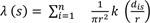
The Fort Peck Reservation is home to two separate Indian nations, each composed of numerous bands and divisions. There are an estimated 10,000 enrolled tribal members, of whom approximately 6,000 reside on or near the Reservation [17]. The reservation is located in the extreme northeast corner of Montana, 40 miles west of the North Dakota border and 50 miles south of the Canadian border, with the Missouri river bordering its southern perimeter [17]. The reservation is 110 miles long and 40 miles wide, encompassing 2,093,318 acres (approximately 3,200 square miles). Of this, approximately 378,000 acres are tribally owned, and 548,000 acres are individually allotted Indian lands. The total of Indian owned lands is about 926,000 acres [18]. Fig. (1) presents the location of the FPIR. The shapefile of the road network was collected from MDT.
The Fort Peck Tribes operate their own transportation program and have a contract with the Bureau of Indian Affairs (BIA) for some transportation functions. Like many other Tribal governments, they work with limited resources to manage and maintain their roadway system. On the FPIR, there are roughly 1,500 miles of roads, of which 375 miles are BIA system and Tribally-owned roads [19]. Of the 211 miles of BIA-owned roads, over half of the roads are gravel and dirt roads. Thus, the majority of the transportation infrastructure under BIA is outdated and in need of an upgrade (paving) while the rest of the infrastructure is owned and maintained by the State and county governments [19].
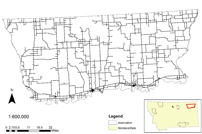
The MDT maintains a crash analysis database for all roadways in Montana. The database includes information on every recorded crash within the state. Crash data within the FPIR was requested from MDT. There were 940 crashes in the FPIR during the years 2005-2014. These include crashes occurring on the state, county, city, and tribally owned roads (Fig. 2).
4. METHODOLOGY
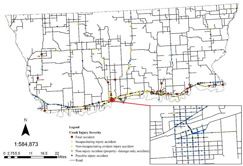
This study used two methods: NetKDE and Getis-Ord Gi*(d) statistics to determine high risk crash locations in the FPIR. Fig. (3) shows the flowchart of the methodology followed to determine statistically significant crash hotspots. This study also performs temporal analysis to assess the crash pattern. The following paragraphs discuss the theoretical background and application of methods.
4.1. Kernel Density Estimation (KDE)
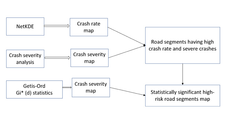
KDE has widely been used for crash hot spots analysis [12]. This method calculates the density of an observed point-event distribution in two-dimensional Euclidean spaces. In other words, the KDE approach calculates the density of neighboring point features around a given point within a circular distance. When represented in three dimensions, the KDE neighborhood bandwidth looks like a bell-shaped curve, symmetrical around the central point feature. The Kernel (or K) function determines the steepness of the curve. A sharper curve generates a more detailed result where a flatter curve yields a smoother density gradient. Adjacent features are provided with a density score based on their distance to the central point. Therefore, the density score declines with the increase of distance. This process is repeated for each point in the dataset. After calculating all the density score neighborhoods surrounding each point, the density scores of the overlapping neighborhoods are added to generate distinct peaks and valleys [20]. Visualized in two dimensions, the result provides a smooth gradient with high and low-density values, which are known as hotspots. The kernel function is presented in Equation 1.
 |
(Eq 1) |
Where, λ (s) is the density at location s, r is the search radius (bandwidth) of the KDE, and k is the weight of a point i at a distance dis to location s. k is usually modeled as a function (called kernel function) of the ratio between dis and r.
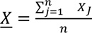
4.2. Network Kernel Density Estimation (NetKDE)
Conceptually, Network Kernel Density Estimation (NetKDE) is an extension of the KDE process. Planar KDE methodology computes density, considering that point events are randomly distributed throughout the Euclidean space. However, traffic crashes do not take place in an open space rather than in roadway networks upon which traffic flows. Therefore, each event has a much stronger influence on their neighbors on the network rather than on a 2-D plane with a constant search radius r. This discrepancy leads to an overestimation bias of up to 20% in planar KDE results when used in a network context [11]. To address this issue, recent researches have focused on the development and use of a KDE in which the neighborhood bandwidth is calculated through a network instead of over Euclidean space. This tool is known as the NetKDE. Instead of computing the density over an area unit, the equation estimates the density of a linear unit. It was first developed by Okabe et al. in 2006 [21] and used in many cases to address the limitation of planar KDE and provide a more accurate interpretation of the distribution of network-bound point events [12]. Fig. (4) presents the difference between the two KDE methods.
4.3. SANET- Spatial Analysis along Networks and NetKDE Analysis
Japanese researcher Dr. Atsuyuki Okabe and his team developed Spatial Analysis along Networks (SANET), an ArcGIS toolbox extension for analyzing spatial events along with network space [21]. In this study, the NetKDE analysis of this toolbox extension was performed on the FPIR crash data layer using the road network database as the network layer. Equal split continuous kernel function was performed as this kernel function minimalizes computation time, particularly when applied on a complex network [12]. Search bandwidth is a critical parameter determining the smoothness of the density results [12]. An optimal search bandwidth in NetKDE should consider both the distribution characteristics of the study area and the road network. In this study, density results were calculated with six different bandwidths of 500 m, 200 m, 100 m, 50 m, 20m, and 10 m. The resulted density values were maximum at 500 bandwidths. The densities vary significantly on different roads and distributed unevenly on the same road, presenting an unbalanced distribution in the entire study area. With the increasing bandwidth, the resultant density values decrease as the denominator “r” increases. As a result, densities change more gently both on different roads and on the same road, and the overall density results get smoother. However, the density values change very little with a 200m, 100m, 50m, 20m bandwidth, which is also undesirable in NetKDE. Therefore, in order to reflect the density distribution variation both on different roads and on the same road, and to keep a balanced distribution at the same time, 10 m of bandwidth length is considered optimal within the study area. Selection of bandwidth 10m was also supported by Xie & Yan (2008) [11], who stated in their study that narrow bandwidths might be suitable for presenting crash hot spots at smaller scales. Cell width was set to 1m, as recommended by the SANET team [21].
4.4. Crash Severity Analysis
Crash injury severity levels include Critical injury, Serious injury, and Property damage only (PDO). Critical injury comprises of fatal and incapacitating injuries while serious injury includes non-incapacitating and evident injuries. To perform crash severity analysis, each crash was assigned a weight based on the ratios of different injury severity level crash costs relative to the PDO crashes. Crash costs collected from the Highway Safety Manual (HSM) [22] were used to determine the weight of each injury level. Table 1 presents the weight assigned to every severity level based on crash cost.
After providing weights to each crash according to Table 1, crash shapefile was converted to a raster file with a cell size of 1 m. Then, the polygon shapefile and road shapefile was merged by using spatial join tools to obtain the road segments with crash severity. Afterwards, the road segments were categorized into three classes. The first category comprised low-risk roads relative to other roads as these roads had no disabling injury or fatality. In the second category, medium risk road segments were made up of more crashes with severe injuries and non-severe injuries than the first category. The last group included road segments with fatal injury associated with other crashes.
To determine street segments and areas of high priority for roadway safety improvements, the results of the NetKDE crash location analysis and crash severity map were compared. In practice, this method was carried out by first dividing the street segments in the NetKDE map into high, medium, and low designations, relative to the values generated through the analysis, similarly as crash severity map. Once this categorization was completed, each respective designation class (high, medium, low) was selected and exported as its layer in ArcGIS. After the six new layers were created, the overlapping segments were highlighted using “select by location” with a 250ft search buffer to include adjacent high-value segments. These highlighted portions were used to create the final map of high risk street segments with a high crash rate and severity. This selection process is similar to the method used by Beckstrom et al. [13].
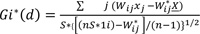
4.5. Getis–Ord Gi * (d) Spatial Statistic
The Gi*(d) spatial statistics method was introduced by Getis and Ord [23] to distinguish between the locations of high and low spatial associations. This tool works by looking at each feature within the context of neighboring features [24]. A feature with a high value may not be statistically significant if it is surrounded by low attribute features. To be a statistically significant hot spot, a feature will have a high value and be surrounded by other features with high values as well [9].
 |
(Eq 2) |
Where, Xj is the attribute value for feature j, Wij is the spatial weight between feature i and j, n is equal to the total number of features and:
 |
(Eq 3) |
 |
(Eq 4) |
In Equation 2, the attribute values of each feature were multiplied by the spatial weight matrix, Wij defines which locations were included in the analysis and corresponding weight. The sum of these observed values was deducted from the expected value, the sample mean. Then, this difference was divided by the standard deviation to obtain a standardized z-score, values for each site i. The Gi* (d) statistics return z-score for each feature in the dataset. For statistically significant positive z-scores, the larger the z-score is, the more intense the clustering of high values (hot spot). For statistically significant negative z-scores, the smaller the z-score is, the more intense the clustering of low values (cold spot) [9]. This study used attribute values as the injury severity type of each crash.
4.6. Conceptualization of Spatial Association
Construction of the spatial weight matrix, or conceptualization of spatial association among the features, is one of the most important aspects of the spatial autocorrelation. Accuracy of the results mainly depends on the ways of interaction between the features. Different methods of conceptualization of spatial relationships, such as inverse distance, inverse distance squared, fixed distance band, zone of indifference, get spatial weights from file, distance band or threshold distance, generate different results [5]. A fixed distance band method was selected for this analysis due to its performance with point features. It is also important to determine a distance threshold associated with maximum spatial autocorrelation because each feature would be analyzed with respect to its neighboring features. In this study, the incremental spatial autocorrelation tool was used to determine the distance associated with the maximum Z score. A distance band of 25,000 m was selected because the minimum distance at which all crashes had at least one neighbor was calculated to be 24,405 m with a maximum Z value of 10.83. Any distance larger than that would result in a larger number of neighbors. Therefore, 25,000 m of distance band would be the best possible option.
4.7. Crash Hotspots Map
Finally, the Spatial join tool was used to join high-risk road segment map generated through NetKDE and other GIS tools, and Map from Getis-Ord Gi* (d) statistics to determine the statistically significant crash hotspots in the FPIR.
4.8. Temporal Analysis, Spider Plot
The temporal analysis enables investigating whether time has an impact on crash occurrences. The time at which crashes occur is crucial to analyze the pattern of crashes and increase infrastructure and emergency response. Spider graph has been used widely to assist in picturing the pattern of crashes over time. As the spider plot has no beginning or end due to its circular nature, it is easier to assess the time interval that is shown discontinuously on the bar chart (e.g. 9 am to 5 pm). Also, only a glance is required to understand the crash pattern throughout the day as the graph resembles a clock.
In this paper, two types of temporal analyses have been performed. The first one is the investigation of the crash pattern throughout the day, and comparison of the temporal distribution of crashes among the three roadway systems, including Indian Reservation Roads, City and County Highways, and State highways. The second one is analyzing the temporal distribution of crash frequency according to the days of the week.
5. RESULTS
This section would outline the results of the discussed methods.
5.1. NetKDE
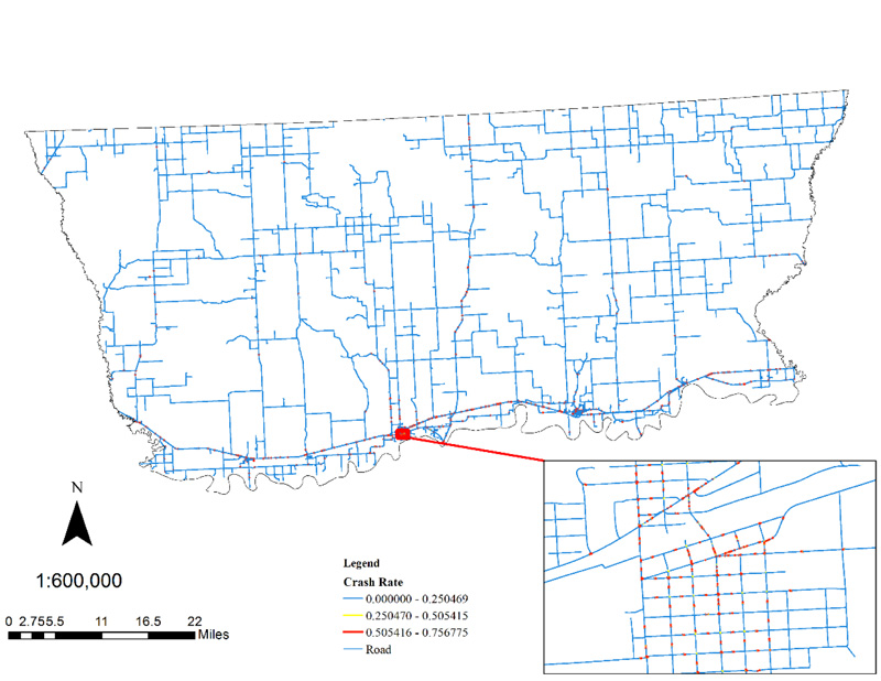
The NetKDE analysis revealed several clusters of crash-prone areas. The result displays a higher degree of linearity due to the network-based calculation. Because of the small bandwidth, high crash rate areas generated the steeper slope. The crash rate map can be found in Fig. (4).
5.2. Crash Severity Map
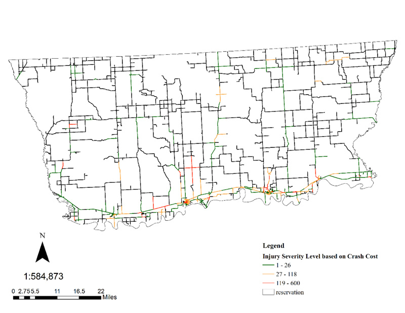
After providing weights to each crash, according to Table 1, road segments were categorized into three classes: low-risk road segments, medium-risk road segments, and high-risk road segments indicated by blue, yellow, and red color, respectively, as shown in Fig. (5).
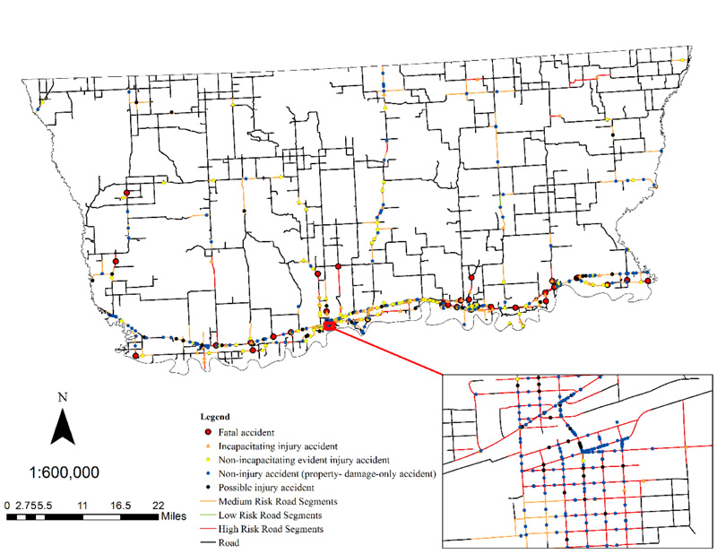
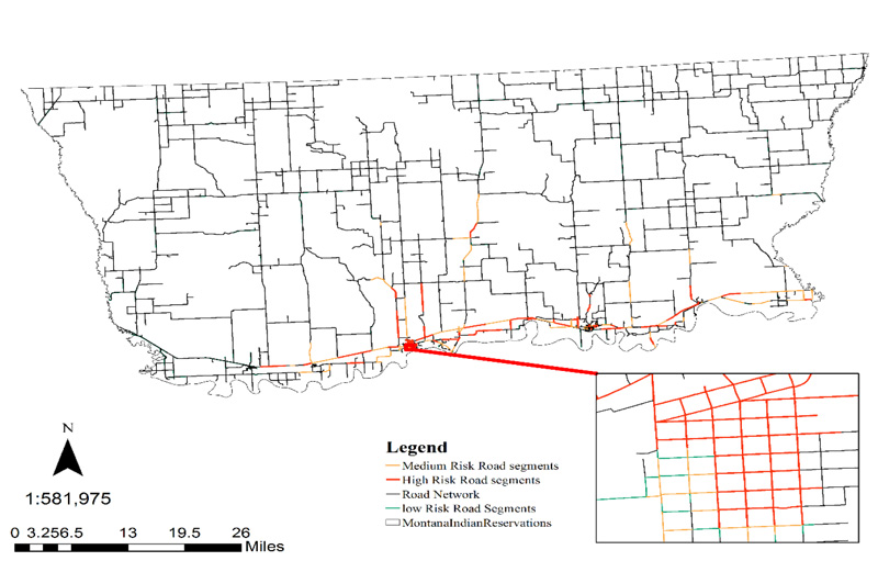
The results of the NetKDE map and crash severity map (Fig. 6) were overlaid to generate a high priority map for ascertaining high risk roads with high crash rate and more severe crashes. The high-risk road segment map, depicted in Fig. (7) presents the results of high-risk road segments. Red color indicates the high-risk road segments, while yellow and green colors represent the medium and low-risk road segments. Some parts of the US highway 13, BIA route 1, and US highway 2 are among the many segments being identified as high-risk road segments in this analysis. Also, although some residential roads have PDO crashes, they have been detected as high priority areas due to high crash occurrence.
5.3. Getis–Ord Gi*(d) Statistics
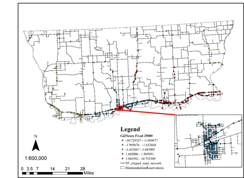
The results of Getis–Ord Gi* (d) statistics analysis of crashes, based on severity level for 10-year period (2005-2014) is presented in Fig. (8). The Gi* (d) statistic provides and negative spatial correlation as the clustering of high and low attribute values. Each crash is represented by a standardized z-score value in five categories, as calculated by the Gi*(d) statistic. The z-score values above and below 1.96 demonstrate crashes that are surrounded by a cluster of relatively high and low weighted values, respectively, statistically significant at approximately 95% confidence level. On the other hand, crashes with a z-score between + 1.96 and −1.96 represent locations that may have a high or low weighted value but are not part of a statistically significant spatial pattern or cluster at 95% confidence level. Fig. (8) shows the result of the hotspot analysis: the red points indicate the locations where accidents with high weighted values are clustered together and the blue points show the locations where accidents with low weighted values are clustered together. In this study, GiZScore of the crashes ranges from -10.73 to -10.75, with GiP Values of 0 to 0.99. The results were interpreted considering the fact that the normal distribution of the variables might not hold true for the crash count [24].
5.4. Crash Hotspots Map
Finally, since NetKDE with crash severity does not show statistically significant road segments, and Getis-Ord Gi* (d) statistics represent statistically significant point features, maps generated through these methods were spatially joined to ascertain statistically significant crash locations. Fig. (9) displays the final map generated through the previous methods. With a limited budget, red-colored /high risk road segments need to be prioritized as most of the crashes with high severity occurred in these road segments.
5.5. Temporal Analysis
Temporal analyses are performed using spider plots. In order to investigate the overall temporal distribution of all crashes, spider plots were generated for a better understanding of the variation of the crashes over time.
5.6. Overall Temporal Distribution
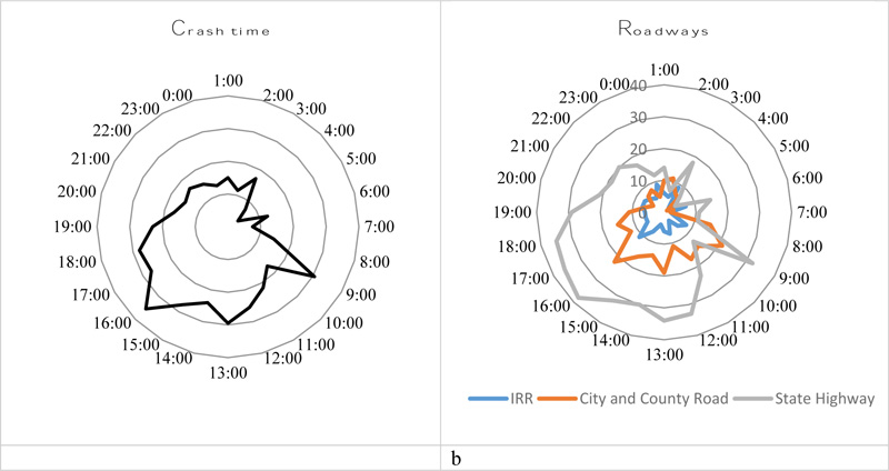
Fig. (10a and b) illustrate how the number of crashes across the FPIR, from 2005 to 2014, varied throughout the day. It is evident that the number of crashes was high at 9:00 am, 1:00 pm, and 4:00 pm, which indicates that most crashes occurred during peak traffic hour. Fig. (10b) shows the crash distribution for three types of roadways: Indian Reservation Roads, City and County Highways, and State Highways. State Highways had higher crash frequency than county roads and reservation roads. While state highway frequency peaks were at 9 am and 4 pm to 6 pm (during peak hour traffic), the crashes on county and reservation roads are distributed throughout the day with the highest frequency at 9 am, 1 pm, and 6 pm. These roads had crashes occuring at midnight (between 12 am and 3 am) when traffic volume is low. Impaired driving is one of the leading causes of crashes on Indian reservations, and may contribute to this high crash occurrences due to its occurrence during night time.
| Injury Severity Level | Comprehensive Crash cost | Weight |
|---|---|---|
| Fatality(K) | $ 4,008,900 | 542 |
| Disable Injury (A) | $ 216,000 | 29 |
| Evident Injury (B) | $ 79,000 | 11 |
| Possible Injury (C) | $ 44,900 | 6 |
| Property Damage Only | $ 7,400 | 1 |
5.7. Days of the Week
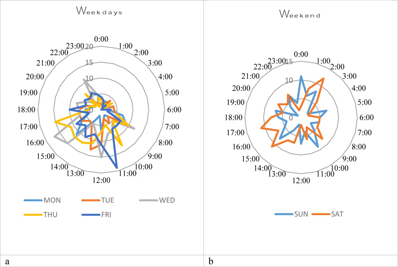
The temporal distribution of crash frequency can also be analyzed by comparing variation according to days of the week, as shown in Fig (11a and b). The figure reveals that the crash distribution over the time of the day exhibits a different pattern on weekdays and weekends. During the week, crashes appear to be more frequent in the morning and evening (11 am-noon and 3 pm – 5 pm), while many weekend crashes occur late in the afternoon (3 pm -5 pm) and early in the morning (12 am to 2 am). There is a large temporal variation from Monday to Thursday. Although crash frequency increases towards the end of the week, crashes are particularly less frequent on Friday, with the highest frequency at 11:00 am. Interestingly, more crashes occurred on Saturday than Sunday. Saturday crashes occurred in the early morning from 12 am to 2 am and afternoon (3 pm -5 pm), which might be explained by the findings of alcohol-related night-time crashes.
CONCLUSION
Crash hotspots were analyzed in an effort to determine the high risk crash locations. A methodology was developed to determine crash hotspots using NetKDE and GIS tools being implemented on the FPIR. This analysis proved to be useful in narrowing down potential locations for improvement, which can then be investigated in their full context for a better risk assessment.
NetKDE was used to locate areas with high crash rates. Then, a crash severity map was generated via a series of GIS analyses in order to determine the locations with the highest severity of crashes. Finally, these two maps were overlapped to ascertain high priority areas that demand immediate attention. This study also employed Getis-Ord Gi* (d) statistic to determine statistically significant crash hotspots. The Getis-Ord Gi* (d) statistic provides positive and negative spatial correlation as the clustering of high and low attribute values.
Each crash is represented by a standardized z-score value, where this z-score values above and below 1.96 demonstrate statistically significant crash hotspots. Finally, maps generated through these two methods were assessed to determine statistically significant high-risk road segments. Also, the temporal analysis of crashes was performed to see the variation of crash patterns throughout the day. The analysis revealed that crash patterns were almost similar on the weekdays reaching the peak at traffic peak hours, but during the weekend, crashes mostly occurred at midnight.
By better understanding where crashes occur, authorities and professionals can decide to utilize funds into areas with the largest impact. This methodology can be adapted in other areas to improve their roadway safety conditions with the marginal investment of resources. Along with the ease of approach, these maps can be used as a powerful visual aid. Tribes will be able to quickly identify the safety concerns without the use of complicated jargons or statistics.
This will help the professionals to incorporate people and create awareness on roadway safety. However, this approach should not be used alone in determining high risk crash locations. Due to the unavailability of traffic volume data, the crash “rate” map generated through NetKDE is actually based on the absolute number of crashes. Since the exposure was not considered in the analysis, the crash rate map might not represent the actual crash scenario in the reservations. Also, there are many other determinants, such as individual behavior, traffic speed, time of day, and weather affecting crash severity and crash occurrence in roadways, and need to be considered during crash hotspots analysis.
CONSENT FOR PUBLICATION
Not applicable.
AVAILABILITY OF DATA AND MATERIALS
Not applicable.
FUNDING
None.
CONFLICT OF INTEREST
The authors declare no conflict of interest, financial or otherwise.
ACKNOWLEDGEMENTS
The WYT2 /LTAP center at the University of Wyoming provided extensive resources to assist in the development of the safety toolkit. The tribal leadership from WRIR and SWO tribes was very supportive and active in its implementation. Special acknowledgment goes to WYDOT and FHWA that provided the resources to make this research possible.

