All published articles of this journal are available on ScienceDirect.

Wheel Slip-based Road Surface Slipperiness Detection
Abstract
Background:
Faced with the high rate of traffic accidents under slippery road conditions, agencies attempt to quickly identify slippery spots on the road and drivers want to receive information on the impending dangerous slippery spot, also known as “black ice.”
Methods:
In this study, wheel slip, defined as the difference between both speeds of vehicular transition and wheel rotation, was used to detect road slipperiness. Three types of experiment cars were repeatedly driven on snowy and dry surfaces to obtain wheel slip data. Three approaches, including regression analysis, support vector machine (SVM), and deep learning, were explored to categorize into two states-slippery or non-slippery.
Results:
Results indicated that a deep learning model resulted in the best performance with accuracy of 0.972, only where sufficient data were obtained. SVM models universally showed good performance, with average accuracy of 0.965, regardless of sample size.
Conclusion:
The proposed models can be applied to any connected devices including digital tachographs and on-board units for cooperative ITS projects that gather wheel and transition speeds of a moving vehicle to enhance road safety in winter season though collecting followed by providing dangerous slippery spots on the road.
1. INTRODUCTION
Road slipperiness is one of the major concerns for road safety. In South Korea, 8,849 traffic accidents that caused 221 fatalities and 13,736 injuries occurred on slippery roads over the three years, which was 27% higher than on dry conditions [1]. In the U.S., slippery roads brought about over 1,300 fatalities and 116,800 injuries, which accounts for 24% of weather-associated road casualties [2]. A study in Sweden indicated that merely 14% of drivers properly accelerate and decelerate on slippery surfaces and 50% of drivers misjudge slippery roads as non-slippery ones [3]. The risk of vehicular crashes and road departures are reportedly nine to twenty times higher on slippery pavements [4].
To reduce the tragic numbers, drivers should be informed of the slippery spots on the road ahead and road managers are required to promptly remove the slippery spots, which emphasizes the need for quick detection of slippery spots on the road. For that, road weather sensors have been conventionally employed [5]. However, as the sensors can only detect an icy point at the road location of the sensor, its utility could be restricted, given that road slipperiness varies even in a short roadway section [6]. Recently, as a growing number of fleets such as trucks, buses, taxis, rental cars, patrol cars, and maintenance cars are getting connected for their own purposes, an innovative approach to identifying slippery spots on the road through processing in-vehicle sensors is attracting interest worldwide.
In this study, a wheel slip-based approach to detect road slipperiness is explored. On slippery surfaces, vehicular wheels are prone to skid, which makes wheel-rotational and vehicle-transitional speeds prominently different from each other. This phenomenon can be discerned by wheel speed and GPS sensors that are available in cars carrying commonly available devices: smartphones, digital tachographs, and on-board units for diverse ITS projects. Due to the characteristics of tires made of rubber, some discrepancies of the two speeds essentially arise for vehicles to move and stop. Hence, finding optimal thresholds of the differences in both speeds that separate skidding from non-skidding under different vehicle dynamic conditions is a principal concern for this study.
The approach suggested in this study has advantages in three aspects: 1) it can be implemented without resorting to sophisticated systems, such as antilock braking and/or traction control systems (TCS) that car manufacturers have normally proprietary rights to; 2) it can be easily applied to any location-based services (LBS) devices enumerated above that include GPS and can obtain wheel speed data from the vehicle’s controller area network bus; and 3) it can provide reliable and spatially seamless slippery information on a wide-area road network when applied to any of the fleets mentioned above, thanks to a systematic analysis on data aggregated from multiple vehicles.
2. LITERATUR REVIEW
Identifying road slipperiness using vehicles as a mobile sensing platform has been one of the hottest research topics for the last two decades. Pilli-Sihvola invented a vehicle-based road weather data collection system to observe road weather data on Finnish roads [7]. Wang et al. developed a vehicle-based tire-road friction estimation system that analyzed data from multiple sensors outfitted in a test vehicle [8]. Nakatsuji et al. proposed a novel method based on a genetic algorithm and the unscented Kalman filter to estimate tire-road friction using vehicle sensor data [9]. Petty et al. tested a potential use of data from Vehicle Infrastructure Integration (VII)-enabled vehicles for road weather-associated applications [10]. Drobot et al. tested a vehicle-based road weather data collection system [11]. Koskinen suggested a technique to estimate the maximum friction while simultaneously diagnosing road slipperiness conditions [12]. Dong et al. developed a method to identify road slipperiness using data from in-vehicle sensors [13]. A pilot project was performed by WyDOT to detect road slipperiness using in-vehicle sensors from multiple commercial vehicles [14]. Hou et al. proposed a system to detect road slipperiness using the acceleration and GPS sensors outfitted in a smartphone [15]. Li et al. proposed an algorithm to estimate tire-road friction using various sensors available in a normal passenger car [16]. Rajamani et al. developed algorithms to estimate independent friction coefficients at each individual wheel of the vehicle using in-vehicle sensors [17]. Mizrachi et al. suggested a method to normalize pavement friction data obtained from multiple vehicles equipped with a specialized device for their project [18]. Du et al. proposed a dynamic method to estimate the pavement friction level using a vision sensor in order to secure the safety of autonomous vehicles on slippery surfaces [19].
Most previous studies utilized proprietary vehicle sensors to identify road slipperiness, indicating that their application could be limited. Although some studies used commonly available sensors included in a smartphone, an arbitrary position of a smartphone in a vehicle undermines their practicability even after correction of accelerometer data based on Euler angles [20]. In addition, several sophisticated methodologies have been developed for vehicular traction controls on slippery surfaces, but their complexities and proprietary features hurt practical applications to connected devices mentioned above. From the perspective of drivers and road managers, whether the road surface is slippery or not is a primary concern. For this reason, a novel but practical method to detect road slipperiness is proposed in this study.
3. METHODS
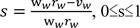
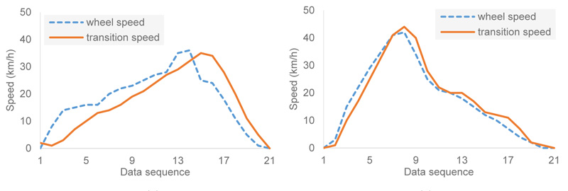
Vehicles have a high risk of skidding during accelerating or decelerating on a slippery pavement. The skidding phenomenon is called wheel slip and can be expressed as (1) One of the practical ways to measure it is to use data from wheel speed and GPS sensors. The wheel slip, the difference between vehicular wheel rotation and transition speeds, on snowy and dry surfaces can be distinctively discerned, as shown in Fig. (1). Wheel speeds, due to the slips, showed higher values while accelerating and vice versa while decelerating. Finding an optimal threshold of the slip that discriminates the pavement states―slippery or non-slippery―is the main purpose of this paper. For that, three methods, including regression analysis, support vector machine, and deep learning, were applied. For all of the three models, wheel slip and acceleration data at one second interval are used for input and road surface conditions (slippery or non-slippery) are generated as output.
 |
(1) |
where s = wheel slip, ww = angular velocity of wheel, rw = effective radius of wheel, vw = vehicular transition speed, and wwrw = wheel rotational speed.
Fig. (2) shows relationships between slips and variables, including the acceleration and speed of the vehicle. No relationship between the slip and the vehicular speed, but strong relationship between the slip and the acceleration, can be intuitively recognized. Hence, the acceleration measurements were used as an independent variable for finding a threshold of the slip to identify slippery pavements.

3.1. Regression Analysis
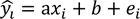
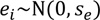
The confidence interval of a regression equation expressed in (2)-(4) can be applied to discriminate slips on slippery conditions from ones on non-slippery conditions. The confidence interval of the i-th estimate can be obtained based on the identical and independent distribution assumption of the error term of the regression equation [21].
 |
(2) |
 |
(3) |
 |
(4) |
where  = the i-th dependent variable (estimate), xi = the i-th independent variable (observation), b = the y-axis intercept, ei = the i-th error, se = standard error of regression line, yi = the i-th observation, and n = number of samples.
Next, thresholds can be determined by (5), where a two-sided confidence interval which includes (1−α)*100% of the wheel slip can be defined with its upper and lower limits for the desired level of false alarm rate (α). A slippery spot on the road can be discernible where any wheel slip outlies the thresholds.
 |
(5) |
where Thr = thresholds of upper and lower confidence interval, N−1 = inverse of normal cumulative distribution function, and α = significance level.
Fig. (3) shows relationships between the slips (unitless) and the accelerations (kph/s) of three types of experiment cars on dry surfaces. Based on the relationships, lower and upper limits at 0.001 significance level can be drawn (see Table 1). All the statistics in Table 1 were proven to be statistically significant by the t-tests. If any observed slip deviates from the confidence interval, it is then classified into a record from the slippery surface. The slips are unitless and the accelerations are in the unit of kph/s.
3.2. Support Vector Machine
Support Vector Machines (SVMs), a sort of supervised machine learning algorithm, are generally used for classification and regression analysis. An SVM model, generally considered a non-stochastic binary linear classifier, constructs an algorithm that allocates new instances to one of two categories for a set of data, each labelled as one category or the other. In an SVM model, instances are represented as points in a space domain, which are mapped for the instances of the separate groups to be divided by the widest gap. New instances are then mapped into the constructed space and categorized to be included in one of the two categories based on the established gap function. Although SVM models are normally applied to linear classification problems, they can also be applied to a nonlinear classification using the so-called “kernel trick” that maps their input instances into high-dimensional feature spaces [22]. In this study, the Python language was used to build a linear SVM model with C value of one for identifying slippery roads.
3.3. Deep Learning
Deep learning, based on Artificial Neural Networks (ANNs), is a sort of machine learning algorithm that utilizes multiple layers to analyze a high level of features from a set of examples. ANNs, inspired by information processing of biological brains, are computing systems with organized communication nodes. Among the learning methods are supervised, semi-supervised, or unsupervised approaches. The term “deep” refers to the number of layers through which features are progressively extracted from the input. In other words, Credit Assignment Path (CAP) is included in deep learning architectures. The CAP is a chain of transformations that connects between input and output. The widely recognized deep learning categories are deep neural networks, recurrent neural networks, and convolutional neural networks, which have been applied to various fields such as image processing, speech/audio recognition, time-series data analysis, where they have resulted in outstanding performances, in some cases, superior to human capabilities [23]. The deep learning model constructed in this study consists of ten hidden layers with ten nodes in each layer with a rectified linear unit function, an adaptive moment estimation optimizer, and the Xavier initializer. To avoid overfitting, a drop-out rate was set at 0.7. Since there is no definite method for selecting optimal number of nodes and hidden layers of deep learning models, the number of nodes and hidden layers for this study were selected with trial-and-error method that revealed the best performance.

| Condition | Sample size |  |
se | Lower (α = 0.001) | Upper (α = 0.001) |
|---|---|---|---|---|---|
| Acc. ≥ 0 | 1800 | 0.84x + 0.01 | 1.55 | 0.84x + 0.01 - (1.55 * 3) | 0.84x + 0.01 + (1.55 * 3) |
| Acc. < 0 | 900 | 0.87x - 0.24 | 1.96 | 0.87x - 0.24 - (1.96 * 3) | 0.87x - 0.24 + (1.96 * 3) |
4. RESULTS AND DISCUSSION
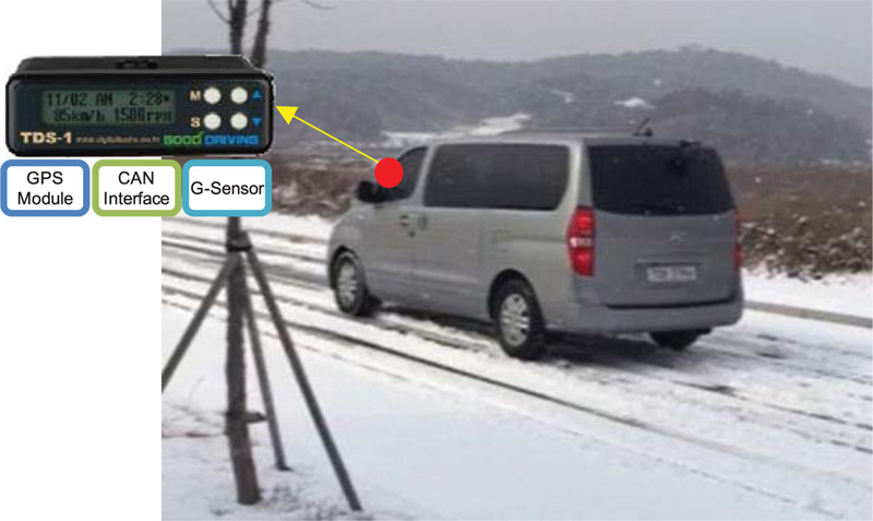
4.1. Data Collection
Data were collected on a specially designed test track with level terrain where adverse weather conditions such as snow, rain, and fog can be arbitrarily created. Three types of vehicles, including a passenger car, a sport utility vehicle, and a recreational vehicle as photographed in Fig. (4), were driven repeatedly on the track when the pavement was dry and covered with snow in January 2019. The experiment conditions were almost consistent because the experiments were performed for about half an hour for dry and snowy conditions, respectively. It should be noted that the purpose of this study is to develop methods for identifying slippery conditions, so it is not necessarily required to maintain the exact same level of slipperiness. Fig. (5) shows the driving pattern of the experiment vehicles outfitted with digital tachographs (DTGs). The driving pattern can be normally observed at intersections where acceleration and deceleration maneuvers repeatedly occurred. The experiment cars’ wheel and transition speeds were recorded on the tachographs on a second basis. In total, 4,122 sets of records were gathered.

4.2. Performance Comparison
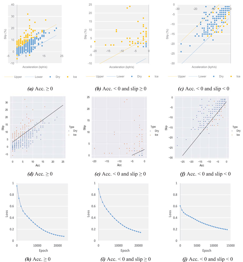
For conducting performance tests on the suggested methods, the experiment data were categorized into three groups according to vehicle dynamic characteristics: 1) acceleration, 2) deceleration with non-negative slips, and 3) deceleration with negative slips. Group 2 indicates that TCSs were activated while stepping on the accelerators, where car speeds decrease even though the accelerators were activated. In each group, 70% of the data were used for training or setting confidence intervals and the remaining 30% were reserved for testing, as represented in Table 2. It should be noted that for testing group 2 by regression analysis, the confidence interval for group 3 was utilized because a regression model for group 2 could not be established, due to a lack of relationship between the slip and the acceleration data of group 2, as shown in (Fig. 6b).
| Group | Condition | Description | Sample size | |
|---|---|---|---|---|
| Training set | Testing set | |||
| 1 | Acc. ≥ 0 | Acceleration without TCS activation | 1800 | 774 |
| 2 | Acc. < 0 and slip ≥ 0 | TCS activated while accelerating | 182 | 80 |
| 3 | Acc. < 0 and slip < 0 | Deceleration | 900 | 386 |
| Group | Condition | Regression analysis | SVM | Deep learning |
|---|---|---|---|---|
| 1 | Acc. ≥ 0 | 0.951 | 0.971 | 0.972 |
| 2 | Acc. < 0 and slip ≥ 0 | 0.955 | 0.962 | 0.924 |
| 3 | Acc. < 0 and slip < 0 | 0.927 | 0.961 | 0.956 |
| Average | 0.944 | 0.965 | 0.951 | |
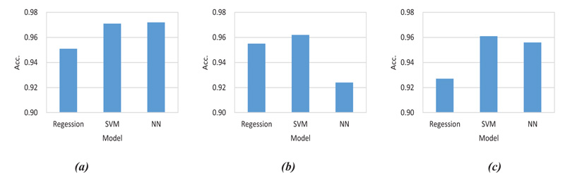
Results, as shown in Table 3 and Figs. (6 and 7), indicated that SVM models revealed universally good performances with an average accuracy of 96.5%, although the highest accuracy of 97.2% was observed when a deep learning algorithm was applied for group 1 where the greatest number of samples were recorded. Regression models exhibited the lowest performances in all conditions, but their simplicity help adoption for embedded systems that normally have an insufficient hardware performance for running machine learning algorithms. The DTG exploited for this study is also a sort of embedded system outfitted in commercial vehicles in Korea. As a whole, the three applied methods showed satisfactory consequences with minor differences in performances.
CONCLUSION
According to a report from the U.S. DOT, around 80% of road accidents could be preventable if drivers have a chance to be informed of the impending dangerous situations on the road ahead [24]. Also, roughly 20% of the road maintenance budget is allocated to winter road maintenance in the U.S. In these regards, road slipperiness detection using connected vehicles can be highly regarded in terms of its low budget requirement as well as the seamless monitoring capability.
In this study, vehicular wheel and transition (ground) speeds were obtained using DTGs, one of the broadly penetrated connected devices in Korea, to calculate wheel slip and acceleration data. After identifying strong relationships between the slip and the acceleration data on dry surfaces, three approaches, including regression analysis, SVM, and deep learning models, were applied to categorize the pavement states-slippery or non-slippery. As a result, SVM models resulted in reasonably good performances with an average accuracy of 96.5%, although the deep learning model showed the best performance for one of the three analysis groups that has the largest sample size.
A follow-up experiment is scheduled in wintertime in 2021 to further investigate that the approach of this study can be applied for data from trucks and buses that carry several kinds of LBS devices for fleet management. In addition, deep learning algorithms need to be further investigated with more data in groups 2 and 3 in Table 2 to find out if the performance of group 1 can be applied to other groups with sufficient data. Lastly, the effect of the road slope for determining thresholds for classifying pavement states needs to be examined.
CONSENT FOR PUBLICATION
Not applicable.
AVAILABILITY OF DATA AND MATERIALS
The data that support the findings of this study are available from the corresponding author (J.J) upon reasonable request.
FUNDING
This work was supported by a grant (No. 19TLRP-B148886-02) from the Korea Agency for Infrastructure Technology Advancement (KAIA).
CONFLICT OF INTEREST
The authors declare no conflicts of interest, financial or otherwise.
ACKNOWLEDGEMENTS
Declared none.

