All published articles of this journal are available on ScienceDirect.

Population vs. Intersection Densities: An Assessment of a Correlation Using Spatial Comparison and Regression Analysis in Yaoundé, Cameroon
Abstract
Background:
Intersection density is associated with block size and positively affects pedestrian volume.
Objective:
This study aimed to show that intersection density and population match across Yaoundé using spatial comparison and regression analysis.
Methods:
For spatial comparison, the mean values of the variables (intersection and population densities) were computed for each administrative subdivision in Yaoundé. The results are reported in a table representing Yaoundé and how the subdivisions share boundaries. For comparison, a table was created for each variable. Simple linear regression with a confidence level of 95% was used for regression analysis.
Results:
Spatial analysis revealed that the pattern of population density was similar to that of intersection density. However, this was disturbed by the proximity to the central business district (CBD). Regression analysis demonstrated that both variables moderately covariate with the influence of CBD. When assuming a weak influence of CBD, they are strong covariates. Statistically, in both cases, the correlation between population and intersection densities did not occur randomly (small p-values).
Conclusion:
The results imply that intersection density is a strong lever that influences citizen behavior. Future planning policies in Yaoundé should consider increasing intersection density in the most crowded areas. It will contribute to the better management of high pedestrian flows in these areas.
1. INTRODUCTION
Street connectivity is the interconnection between streets and the density of intersections. It has been widely discussed in the literature, particularly in matters related to space syntax (the set of methods for analyzing human activity patterns in urban blueprints). Its usefulness has been demonstrated in urban sciences to assess walkability in cities and the health field [1-7]. However, it has been found that connectivity can be poorly related to walkability in certain cities [8]. This outcome differed from those obtained from studies conducted in urban areas in the Western world.
In some studies, intersection density (the number of intersections in an area) is used instead of street connectivity to measure walkability. The greater the intersection density, the greater the walkability would be. Ewing, Reid, and Cervero evaluated the built environment metrics of 50 academic sources (these included population density, diversity, and design, which included intersection density, destination accessibility, and distance to transit) and concluded that intersection density is the one most related to walkability [9]. This result contradicts the findings of Peponis et al. [8], who found that population density was more related to walkability. The extent to which intersection and population densities relate to each other remains unclear. Nevertheless, both have been used together to correlate with other parameters, such as walking [10]. However, no cause-effect interaction between them has been established: who impacts the other, population or intersection density?
The present study aimed to establish a correlation between the intersection and population density in Yaoundé. The study hypothesizes that these metrics have similar patterns across the urban fabric and that one of the parameters influences the other. Population and intersection densities were studied in Yaoundé using a spatial comparison using Geographic Information System (GIS) maps with a resolution of 1 km to prove their intercorrelation. The mean values of both densities were calculated for each administrative division in Yaoundé. The variation in the mean values from one administrative division to another was obtained for the intersection and population densities. Comparing the population and intersection densities mean variation showed that the studied metrics shared similar spatial patterns in Yaoundé.
2. LITERATURE REVIEW
Population and intersection densities are two common urban metrics in the study. Before discussing this in detail, it is useful to know more about the metrics. Studies have created and adopted numerous parameters called urban metrics to classify urban areas according to their forms and functions. These metrics can be spatial, social, or economic. This study aims to obtain an inclusive list of metrics and determine which are more relevant. Ewing and Cervero classified metrics as density (household density, population density, and job density), diversity (land-use mix, job/house balance), design (intersection and street densities), destination accessibility (job accessibility by auto, transit, and distance to downtown), and distance to the nearest transit stop [9]. The authors emphasized elasticities, which are the “ratios of the percentage change in one variable associated with the percentage change in another variable.” With regard to walking, intersection density showed the greatest elasticity. This means that high intersection density is positively related to high walkability. These metrics are useful for quantifying urban phenomena such as sprawl Jaeger et al. defined sprawl as a visually perceived phenomenon in a landscape [11]. Torrens summarized the attributes of urban sprawl found in the literature between 1990 and 2003 [12]. These attributes are growth, social, decentralization, accessibility, density, open spaces, dynamics, costs, and benefits. Among these characteristics, density was the most common. In the assessed studies, density was measured using many metrics. Among these are density metrics (gross population density surface, population density surface considered over developable land, and population density profile as a function of accessibility to the central business district [CBD]). The attributes of sprawl are not the only frames used to measure city expansion. Angel et al. distinguished between the attributes and manifestations of sprawl [13]. As there are many types of sprawls, attributes describe all types of sprawls, but manifestations are specific to a certain form of sprawl. The third concept is associated with the spatial transformation of cities: dimensions. The dimensions of sprawl include eight urban attributes (density, continuity, concentration, clustering, centrality, mixed uses, and proximity), whose combination expresses the type of sprawl [14]. Logically, they can also express urban forms. When measuring sprawl, it can be seen that density is broadly used as a metric. Second, intersection density does not appear as a metric. However, the percentage of the built-up area used as sprawl manifestation metrics is somehow linked to intersection density. (Density metric is closely related to the size of urban blocks.)
Intersection density is the number of intersections per unit area. The greater the intersection index, the smaller the block size. The smaller the block size, the greater the walkability. Walkability is very important for access to amenities. The walkability index established by Franck et al. was computed using intersection density and other parameters, such as net residential density, retail floor area ratio, and land use diversity [15]. A walkability score based on the walkability index has been reported in the literature. Numerous authors have discussed these points. Frank et al. compared two other walkability evaluation methods: the walkability index and the original airline walkability score (OA-WS) [16]. All three methods rely on the intersection index. Frank et al. found that the walkability index remains the best method for estimating walkability [16]. Higher walkability (higher street connectivity) contributes to reducing greenhouse gas (GHG). Hajrasouliha and Yin addressed the effect of street connectivity on pedestrians [17]. They concluded that the higher the street connectivity, the higher the pedestrian flow. A higher number of pedestrians means less GHG emissions. Nevertheless, the results obtained by the authors were possible because of the action of other factors, such as land-use diversity and job population densities.
Population density is the number of people per unit area. Population density functions have been a focus of studies since the 1950s because of their interest in economics [18-20]. Estimating population density across a given area provides a better understanding of the area’s social and economic assets [21]. Population density functions have been developed for this purpose. Such functions provide the population density at a certain distance from the CBD. Theories on population density can be found in studies by Mills and Tan [18]. Interest in describing population density with functions was more visible between the 70s and the 80s. Nevertheless, these contributions will be discussed later by some researchers. In the early 1990s, Batty and Sik Kim proposed the inverse exponential as the best description of population density [22]. Apart from studying its distribution, population density intervenes in understanding social and geographical phenomena, such as the sprawl mentioned earlier. The next paragraph discusses the connection between population and intersection densities when describing such phenomena. Intersection and population densities have been used to describe many urban phenomena. These phenomena include human activity [23], obesity [24], and road accidents [25]. These studies used intersection and population densities as variables with other quantities. However, few studies have directly related population density to intersection density.
The present literature review shows that studies on intersection density focused most on how walkable an area is (walkability index) and questions related to walking activities such as health and safety. This study's research on intersection density was extended to include its direct correlation with population density. Such a correlation could induce the use of intersection density to influence the behavior of citizens.
3. METHODOLOGY
3.1. Area of Study
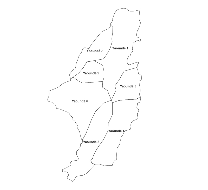
The study area is Yaoundé. Yaoundé is the capital of Cameroon and the central region. It is located 200 km from the Atlantic coast, between 4° North latitude and 11°35 East longitude. It is surrounded by seven hills that are responsible for its particular climate. The city's foundation began with Jaunde Station, a German military post constructed in 1889. Currently, the area of the city is 304 km2, with only 182 km2 being urbanized. Yaoundé is administratively divided into seven municipalities: Yaoundé 1, Yaoundé 2, Yaoundé 3, Yaoundé 4, Yaoundé 5, Yaoundé 6, and Yaoundé 7 (Fig. 1). The Yaoundé City Council heads all these municipalities. Shapefiles of the administrative division of Yaoundé were obtained from the Cameroon data grid on the website of Humanitarian Data Exchange (HDX). The United Nations Office owns the HDX for the Office for the Coordination of Humanitarian Affairs (OCHA).
3.2. Obtention of Population Density Data
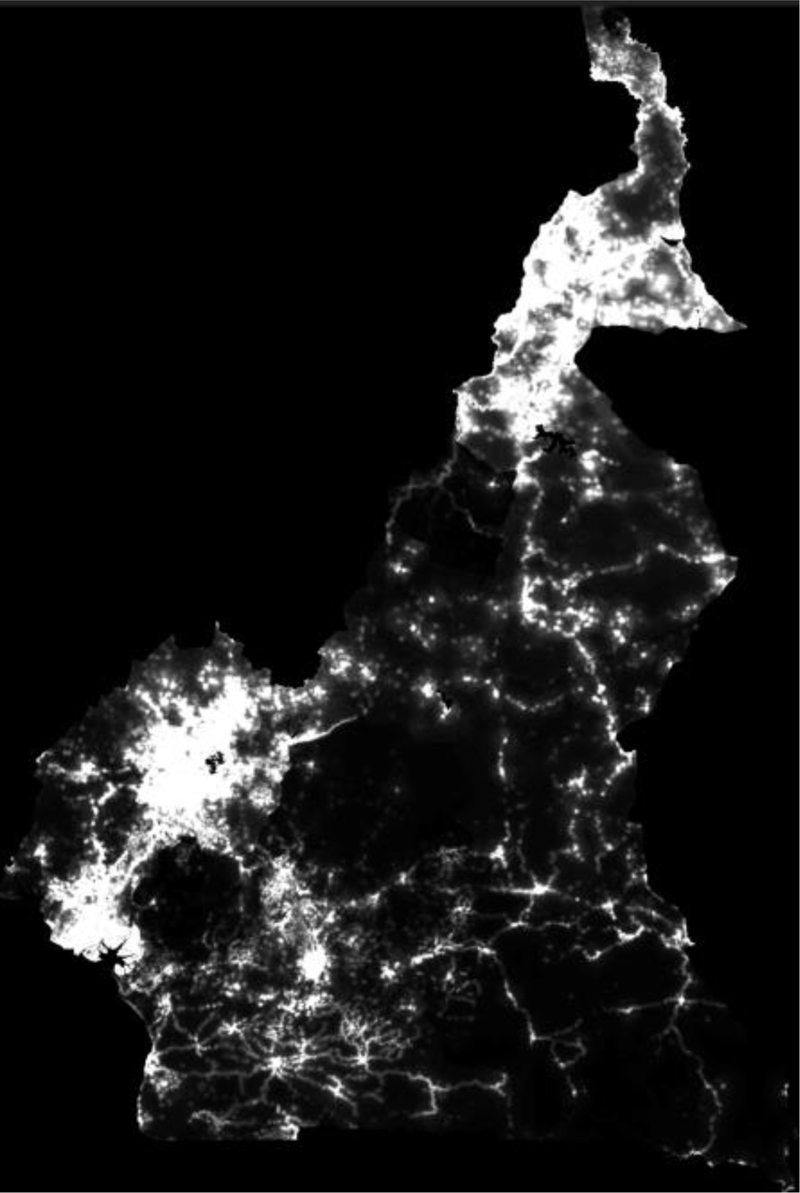
Raster images of the Cameroon population density for 2020 were downloaded from the WorldPop website. WorldPop produces GIS maps of population counts and densities. Mapping is performed using constrained or unconstrained top-down modeling. While constrained modeling relies on built-up areas to provide more accurate mapping (population is null where there are inhabited areas), unconstrained modeling can do so without construction distribution. In this study, unconstrained mapping of the population was used. Unconstrained modeling has the disadvantage of allocating populations to inhabited areas. Nevertheless, the density in inhabited areas with unconstrained modeling is very low, and this disadvantage can be minimized. The resolution of the raster images provided by WorldPop is 30 arcseconds, which corresponds roughly to 1 km at the equator. The population density inside the Yaoundé administrative boundaries was clipped using QGIS 3.22.
Fig. (2) shows the gray shade map of the population density of Cameroon in 2020, as downloaded from the WorldPop website. The brighter the area on the map, the higher the population density. Black areas inside the territory of Cameroon indicate a population density of zero. This is the case with water surfaces.
3.3. Intersection Density
The street network of Yaoundé City was extracted in QGIS (Quantum Geographic Information Systems) from the Open Street Map (OSM), whose precision is very close to that of highway mapping. Intersection density was then computed from the street network. The entire process for the computation of intersection density is described on qgistutorials.com. The intersection is broadly understood here as where two or more roads or streets meet and cross. This term encompasses all the junctions (two or more roads meet, and in the case of two roads, one continues going on) like intersections in the strict sense (an at-grade junction, which means that meeting and crossing are done at the same level), interchange (a grade-separated junction, which means that meeting and crossing are done in at different levels), and roundabout (a circular type of junction where traffic run in one sense with particular priority rules for vehicles). While measuring the intersection density in QGIS, no distinction is made between the types of junctions. It is important to note that OSM updates its data regularly, whereas WorldPop provides data from 2000 to 2020. Consequently, there is a difference of two years between the street network map extracted from the OSM (2022) and the population density map of WorldPop (2020). However, the gross population density (the ratio of the entire population to the area of the city) of Yaoundé between 2020 and 2022 passes from 21,936 inhabitants/km2 (3,992,441 inhabitants divided by 182 km2) to 23,829 inhabitants/km2 (4,336,670 inhabitants divided by 182 km2), this difference in years was neglected. (The relative difference is 0.086.)
3.4. Spatial Comparison: Population vs. Intersection Densities
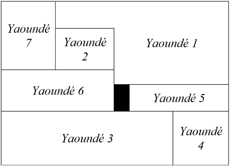
For spatial comparison between population and intersection densities, the administrative division of Yaoundé was used (Yaoundé 1, Yaoundé 2, Yaoundé 3, Yaoundé 4, Yaoundé 5, Yaoundé 6, and Yaoundé 7). For each division, the mean value of the population (and intersection density) was calculated using the QGIS. Population and intersection values were classified by defining class modes using equal counts (i.e., class intervals have the same number of values). For the population density map, which was a raster shapefile, polygonization from the raster to the vector file was necessary to extract the mean values per division. The results are then presented in a table (Fig. 3), imitating the city administrative divisions of Yaoundé (a tabulated city). Each tabulated division is colored as a function of its mean value in compliance with the spectral color ramp classification conducted in the QGIS software. (For mean values ranging from the lowest to the highest, the color ranges from blue to red). A tabulated city was created for population density and another for intersection density. The variation in mean values from one tabulated division to another was compared for both densities. Correlation and regression analyses verified the results of this comparison.
3.5. Correlation Analysis
Correlation analysis was used to determine the extent to which a variation in intersection density induces a variation in population density. Pearson’s correlation coefficient was used for this purpose. Table 1 shows the relationship interpretation.
| Correlation Coefficient (Absolute Value) | Relationship Interpretation |
|---|---|
| 0.000–0.199 | Very weak |
| 0.200–0.399 | Weak |
| 0.400–0.599 | Moderate |
| 0.600–0.799 | Strong |
| 0.800–0.999 | Very strong |
| 1.000 | Perfect |
3.6. Regression Analysis
Simple linear regression analysis with a confidence level of 95% was chosen to evaluate the significant effect between intersection and population densities. A scatter plot of the mean values of intersection density versus the mean values of population density in the Yaoundé subdivisions was constructed. The best-fitting regression line was obtained by minimizing the residuals using the least-squares method. Attention was paid to the p-values at the end of the analysis. The p-value was useful for determining whether the null hypothesis (random correlation between intersection and population densities) would be adopted or rejected. The p-value should be less than 5% to reject the null hypothesis.
As the distance to the CBD influences people’s settlements, two cases were assessed for the regression analysis. The first case assumed a significant influence of the CBD by considering all subdivisions of Yaoundé. The second case assumed the influence of the CBD by considering only subdivisions where the population gradient was very low (considering an equal interval mode classification in QGIS). A population gradient equal to zero means that the proximity of the CBD does not perturb the population's repartition. In other words, the population was assumed to be uniformly distributed throughout the city.
4. ANALYSIS
4.1. Cells Data Collection
The computations of the intersection and population density values were performed separately. The vector files obtained had the same resolution; however, their cells did not overlap perfectly, even after merging them in the software.
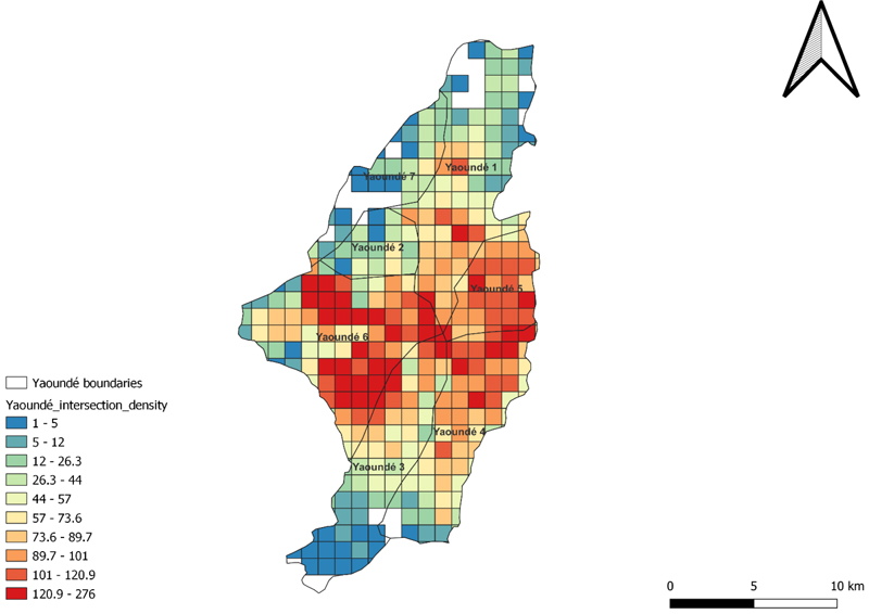
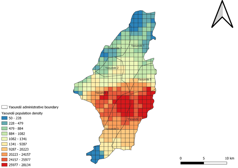
Regression analysis was performed considering the population and intersection density values stocked in the cells. The mean values in the Yaoundé subdivisions were insufficient because the regression analysis required a number of observations that were high enough to provide a certain accuracy. The area of each cell corresponds to the resolution of the maps (1 km × 1 km). It was necessary to ensure that the value of a cell on the population density vector map was collected together with the value of the corresponding cell in the intersection density vector map. However, the cells did not match perfectly. Despite matching the administrative boundaries of the maps, a shift was observed between the cells of the intersection density map (Fig. 4) and those of the population density map (Fig. 5). Moreover, the resolution of the intersection density was not exactly 1 km but approximately 1 km (30 arcseconds). Therefore, the number of cells on the population density vector map might differ from that on the intersection density vector map.
Both maps were opened together in QGIS with the population density vector layer over the intersection density to solve this issue. The cell values are displayed for both maps. The screen scale was set to 1:25,000, which was optimal for collecting the intersection density and population values of the cells. Data were collected on the QGIS screen (from the perspective of the population density map displayed because it was over the intersection density map) and reported manually on a Microsoft Excel sheet using this scale. It was done by considering only the cells where the population and intersection density values were displayed together. It means that the first errors were avoided (as some cells showed two values of intersection density and others no value of intersection density). The intersection value collected was in the neighborhood of the corresponding population density value, and every intersection density value was collected with its corresponding population density value. However, this process is time-consuming and requires the concentration of the person to collect data to minimize errors. Table 2 presents the number of values collected with respect to the total number of cells.
4.2. Assumptions for Regression Analysis
The assumption considered for the regression analysis (influence of the CBD and weak influence of the CBD) depends on the location of the cells in the vector map. In the case where the influence of CBD is considered, all cells are considered. It is because it is assumed that the CBD influences the population pattern anywhere in Yaoundé. This situation is depicted in Fig. (6), where the population gradient (the variation in the population with respect to the distance to the CBD) increases from the boundaries of the city to the CBD (the red hotspot).
| Variable | Number of Cells on the Vector Map | Number of Cells Collected | Percentage of Cells Used |
|---|---|---|---|
| Population density | 440 | 297 | 67.5% |
| Intersection density | 352 | 297 | 84.4% |
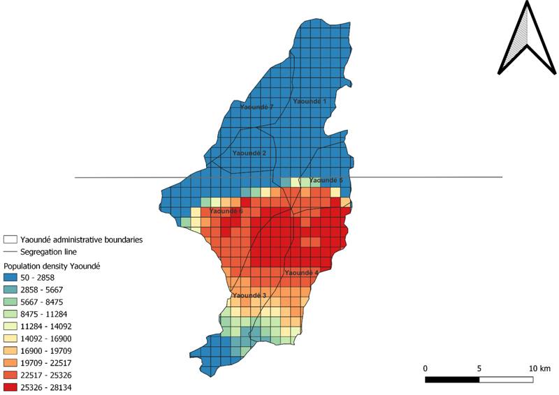
The case in which the influence of CBD is neglected necessitates analyzing from another perspective. As shown in Fig. (6), the population density values were classified by defining the class mode using equal intervals (i.e., intervals have approximately the same amplitudes) instead of using equal counts in QGIS. It is possible to determine which values are within the same interval with this classification. Cells above the segregation line in Fig. (7) (125 cells) were chosen for this case.
5. RESULTS
5.1. Spatial Comparison
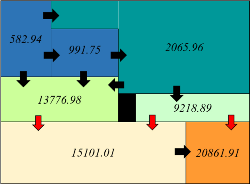
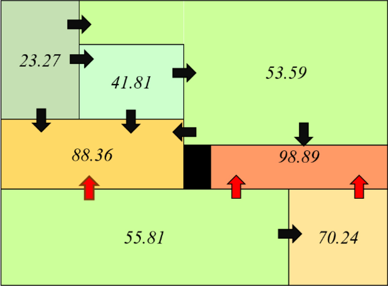
A tabulated form of the city was obtained for the population and intersection densities. In these tabulated city forms, arrows were used to show increasing variation between two adjacent subdivisions of Yaoundé. Black arrows indicate that the variations are identical for population and intersection density maps. In contrast, the red arrows indicate that the direction of the variation in one map is opposite to that of the variation on another map.
Figs. (7 and 8) show that only three arrows are red. These arrows are directed downward for population density and upward for the intersection. The interpretation of this result is that population and intersection densities follow the same pattern. However, the downward direction of the red arrows in the population density-tabulated city indicates that individuals follow something other than intersection density: the CBD. Indeed, the CBD of Yaoundé is in Yaoundé 3 (population density of 15,101.01, intersection density of 55.81).
5.2. Population vs. Intersection Densities: Influence of the CBD
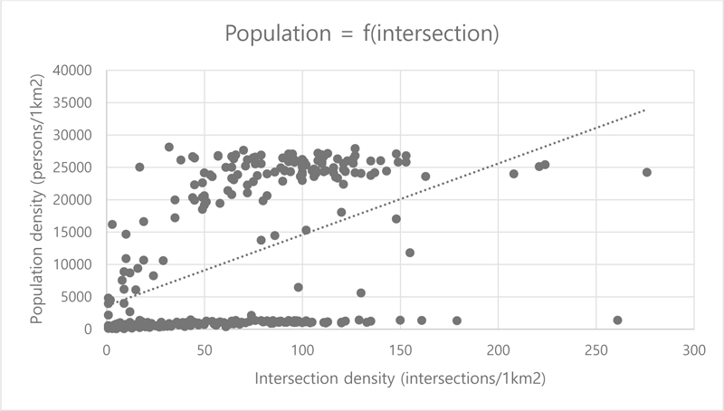
Fig. (9) shows the scatter plot of population versus intersection densities when considering the influence of the CBD.
The regression analysis performed in the Microsoft Excel data analysis tool showed a p-value of 7.65×10⁻¹⁸ (with a confidence level of 95%, 297 observations). The null hypothesis (random relationship between variables) was rejected with a confidence level of 95%. However, the value of R2 is 0.222, which means that under the influence of the CBD, intersection density accounts for 22.2% of the choice of housing location by people. The correlation coefficient R is 0.471, which indicates a moderate relationship between intersection and population densities. The regression line equation is given in Eq 1.
 |
(1) |
5.3. Population vs. Intersection Densities: Weak Influence of the CBD
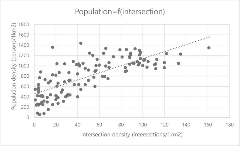
Fig. (10) shows a scatter plot of population versus intersection densities when considering the weak influence of the CBD. The dispersion of points permits the expectation of a strong relationship between population and intersection densities.
For this case, with a p-value equal to 1.49×10⁻²³ (with a confidence level of 95%, 125 observations), the null hypothesis (random relationship between variables) is also rejected. The value of R2 is 0.558. The value of the correlation coefficient R was 0.746. Thus, the relationship between intersection and population densities is strong. The regression line equation is given in Eq 2.
 |
(2) |
6. DISCUSSION
The findings of the analysis demonstrate that population behavior in housing choice is influenced by two variables: distance to the CBD and density of intersections. A higher intersection density ensures greater mobility for citizens and better access to amenities. Because the CBD provides most amenities, populations are more likely to prioritize housing close to the CBD. Consequently, certain areas of Yaoundé became more crowded while the number of intersections slowly increased. Table 3 shows that Yaoundé3 (home to the CBD), Yaoundé4, and Yaoundé6 are crowded with respect to other subdivisions.
| Yaoundé1 | Yaoundé2 | Yaoundé3 | Yaoundé4 | Yaoundé5 | Yaoundé6 | Yaoundé7 |
|---|---|---|---|---|---|---|
| 0.026 | 0.042 | 0.004 | 0.003 | 0.010 | 0.006 | 0.040 |
The information in Table 3 can be explained through Yaoundé’s history. The first urban perimeter of this city was defined during the French colonial period (1916–1960). The first perimeter was built around the CBD. Colonial planning of the city CBD will be maintained during the next few decades. Between 1960 and 2000, a second nucleus was built during the colonial period. Since 2000, urbanization has accelerated, and people have settled in urban peripheries, many coming from the inner part of the city. Land availability and housing prices mainly provoke the displacement of people to the outskirts of the city. Despite this displacement, the CBD remained the most crowded as the population increased naturally, and people migrated from rural to urban areas for work, studies, commercial activities, and so on. Workplaces (particularly administrative works), notorious high and advanced education establishments, and big commercial centers of Yaoundé gravitate around the CBD.
CONCLUSION AND RECOMMENDATION
Previous studies have shown a correlation between intersection density and walkability. Many walkability indices are computed based on intersection density [15, 16]. However, little attention has been paid to the relationship between intersections and population densities. This study established this relationship in Yaoundé by minimizing the influence of the CBD and using spatial comparison and regression analysis.
The pattern of the population follows that of intersection density. A spatial comparison shows that the proximity of the CBD perturbs this pattern. Considering the influence of CBD, the relationship between the two variables was moderated. Assuming a weak influence from the CBD, the relationship is strong. This finding is consistent with that of Hajrasouliha and Yin [17], who found a positive relationship between intersection density and pedestrian flow. Indeed, a large pedestrian flow implies a large population. In addition, the study has a contribution: the dependence of population density functions not only on the distance to the CBD but also on the intersection density. Therefore, planning policies should also be oriented toward laying out a sufficient number of intersections to improve mobility for the city or to use this number to impact citizen behavior in their choice of housing location.
As virtually no studies have mentioned a direct relationship between population and intersection densities, the present study is characterized by its novelty. The impact of street layouts on people’s behavior has been well discussed in the literature. In this study, a new stone was created to design a layout considering the population density forecast. However, this study had some limitations. First, although small p-values supported the analysis, the findings are not strong enough, as they need to be obtained in other cities. Thus, future studies should focus on establishing a strong relationship between population and intersection densities or showing that this relationship is valid only in certain cities. Second, no distinction was made between the type of junctions in the present study. Carrying out the analysis by considering different types of junctions could lead to different findings. For instance, in Yaoundé, intersections in the strict sense (at-grade junctions) are more numerous than roundabouts, mainly found in the CBD area. Third, accessible data with a degree of accuracy fair enough were used. The study would perhaps deserve to be repeated with more recent and accurate data through methods like in situ censuses for population density and inspection of high-precision satellite images for intersection density.
In Yaoundé, the diminution of the intersection/population ratio when moving from the outskirts to the CBD can explain traffic management and mobility problems. Moreover, the city was not sufficiently walkable. Planning decisions should aim to increase the number of intersections, particularly in the most crowded areas, to allow drivers and pedestrians to avoid congested sections when attempting to reach specific destinations. A high intersection/population ratio also contributes to an increase in walkability and a decrease in GHG emissions, provided sufficient sidewalks are laid out and pedestrian management equipment (crosswalks and traffic lights) are in place.
LIST OF ABBREVIATIONS
| CBD | = Central Business District |
| GIS | = Geographic Information System |
| OA-WS | = Original Airline Walkability Score |
| GHG | = Greenhouse Gas |
| OCHA | = Office for the Coordination of Humanitarian Affairs |
| QGIS | = Quantum Geographic Information Systems |
| OSM | = Open Street Map |
CONSENT FOR PUBLICATION
Not applicable.
AVAILABILITY OF DATA AND MATERIALS
The data and supportive information are available within the article.
FUNDING
This study was supported by the Ministry of Education of the Republic of Korea and the National Research Foundation of Korea (NRF-2020S1A5C2A01092978).
CONFLICT OF INTEREST
The authors declare no conflict of interest, financial or otherwise.
ACKNOWLEDGEMENTS
The authors acknowledge the support of the Ministry of Education of the Republic of Korea and the National Research Foundation of Korea.

