All published articles of this journal are available on ScienceDirect.

Estimation of Cross Classified Value of Travel Time Using Binary Logit Model on Egyptian Roads
Authors Info & Affiliations
Abstract
Objective:
In this study, cross-classified categories of Value of Travel Time (VOT) are estimated using the binary logit model for the users of both public and private vehicles who have diverse income levels and go on different trips. The travelers’ income level has a large impact on their VOT and on their willingness to pay regarding other factors that impact the travelers’ choice of the most suitable means of transport for them.
Methods:
The research uses the combined stated and the revealed preference survey and applies the logistic regression analysis to estimate the categorized VOT on Egyptian roads. The data sets consist of 1123 respondents who were approached to collect information related to the socio-economic factors and the trips’ characteristics. Each respondent was requested to choose an alternative to each of the choice sets’ levels. All data sets were collected in light of the Binary Logit analysis and recorded concerning the socio-economic factors. A total of 33 models were developed to predict the VOT.
Results:
According to the given analysis, VOT for private car owners (32.5 LE/HR about 2.06 $/ HR) is higher than that for public transport users (18.3 LE/HR about 1.16 $/ HR) in Egypt. As for the diverse income level groups, a positive correlation is found between each traveler and his/her income. To clarify, the travelers’ VOT increases when their income levels improve.
Conclusion:
Concerning the purpose of the trip, the VOT reaches its peak for travelers who travel for the sake of work as their VOT is approximately 38.82 LE/HR, about 2.47$/HR compared to the other travelers who have different traveling purposes other than doing business.
1. INTRODUCTION
Regarding the transportation field, studies show that travelers who value their time have shown a willingness to pay more money to reduce the amount of time spent on their traveling; however, there are indeed several crucial factors that influence their decision of paying more money. For instance, the travelers’ objectives, the duration of the trip or its length, and the character traits that differ from one individual to the other are the most significant factors. As a result of such factors, each individual would have his VOT and it is uncommon for different travelers to have similar VOT. The significance of reducing travel time is embodied in three main concepts. The first concept revolves around replacing the time wasted in traveling with another activity that would give either the travelers or their employers a monetary gain. The second concept suggests replacing the time wasted in traveling by doing some sort of entertaining activity, or in doing an appropriate recreational activity for those who can afford it. The third concept states that the traveler might face discomfort, stress, or exhaustion during the trip. Accordingly, reducing the time spent traveling would be more beneficial to the traveler.
The quantification of VOT is based on the data collected from surveys to establish models, followed by the cost coefficients and the time used for the estimated VOT. Three levels of cross-classification matrices have been used to describe the relationship between VOT and travel modes, VOT and different income levels, and VOT and travel purposes. This paper uses logistic regression analysis to build models for the estimation of VOT and shows its application on Egyptian roads. The author [1] first puts forward the idea of VOT using 1965’s discrete choice modeling which was based on random utility theories. In the following decades, after the sixties, the development of computers continued to promote such research. As for the analysis of this research, the Statistical Package for Social Sciences (SPSS) was used and several Excel Macros were developed as well [2].
The structure of the paper is as follows: The first section includes a summary of related literature, while the next section gives an overview of the application methods and the methodology of this study. Both sections are followed by highlighting the specification of the model and the outcomes of estimating the entire data. The last section sheds light on the conclusions of this study, along with giving some recommendations for further research.
2. LITERATURE REVIEW
Concerning the principle of VOT, delay and travel time can be transferred to cash amounts, but VOT is a very dynamic measure that depends on many parameters and changes that differ from one country to another and from one person to the other. In terms of data collection and the models used, the purpose of this literature review is to present the latest technology utilized for modeling VOT.
Many efforts have been made in the past, with the international value of time review studies [3, 4] reporting values utilized in various countries and road jurisdictions. Some of these studies were conducted at the national level in many countries such as the United States, the United Kingdom, Sweden, France, and others as localized studies for specific projects such as expressways, tolls, and many small scales report studies to estimate VOT values and clarify their variation across different variables, to improve and make a cost-benefit analysis and forecasting procedures more pragmatic.
Individual studies have also made several efforts to analyze VOT variance over multiple subgroups of variables such as diverse income and distance bands, different travel reasons, gender, and so on.
Various approaches for calculating monetary VOT have been established based on average wage rates or willingness-to-pay (seen behavior of people who sell time for money and research to evaluate people's value of time savings).
According to the current AAHSTO standards, the standard value for travel by car and bus is 50% of the wage rate, which is increased to 70% for personal automobile travel to represent the positive distance elasticity. Waiting, walking, and transfer time is all worth twice as much, and corporations payout 100% of their total compensation for travel.
Considered experimental data gathering approaches such as stated preference, as well as results based on the typical revealed preference method, an example of willingness to pay to estimate VOT. A study [5] employed a combination of revealed preference (RP) and stated preference (SP) data to analyze passenger choice behavior regarding the use of restricted lanes (MLS). The data was taken from the South Florida Expressway, and an average value for VOT and VOR was calculated using mixed logit modeling. Using a poll of stated preferences, the value of travel time in Nanjing is evaluated [6]; respondents are offered six expressed preference questions for each trip purpose.
In terms of estimating VOT for different trip purposes, Stated preference (SP) survey data for Beijing were collected to approximate VOT for those who traveled for business and leisure purposes under various circumstances [7]. To approximate a particular VOT for leisure journeys [8], uses real driving options between open access and toll roads to perform a Monte Carlo simulation to define generalizable outcomes for subsequent valuation studies. Furthermore, the authors [9] estimated Using a dataset on the respondents' time-use and spending allocation for a one-week reporting period, the value of leisure (VoL), the value of travel time savings (VTTS), and the consequent value of time assigned to travel (VAT) for workers in the Canton of Zurich, Switzerland.
To calculate VOT, various models have been developed [10] to estimate the value of travel time savings for Japanese road users when choosing between an expressway and a non-expressway route using a standard binary logit and a mixed binary logit model, the mode choice approach to assess the significance of time by distributing questionnaires to travelers was used in a study [11]. The method is used to estimate these figures using groupings of cars that are used on weekdays and weekends. The Binary Logit model was developed to approximate the importance of travel time for different income levels as well as varied journey lengths in the form of individuals traveling to work during the morning cycle in the Calicut region [12].
3. MATERIALS AND METHODS
Regression analysis is a type of predictive modeling technique for evaluating the relationship between one or more independent variables (the “X” variable) and a dependent variable (often referred to as the “Y” variable). When two or more independent variables are used to predict or explain the outcome of the dependent variable, this is known as multiple regression.
Linear regression and logistic regression are the two major methods of regression analysis. For predictive analysis, linear regression is commonly employed in statistics. It essentially determines the degree to which a dependent variable and one or more independent variables have a linear relationship. Linear regression produces a trend line shown among a group of data points as an output.
Logistic regression is the second form of regression analysis. It is the chance of something happening that is calculated (or predicted) using logistic regression analysis.
Three purposes can be served by regression analysis:
1. Predicting the consequences or consequences of specified changes.
2. Predict future trends and values.
3. Assessing the impact of independent variables on a dependent variable (or, in other words, determining the strength of distinct predictors).
Logistic regression is a solution for grouping. The logistic regression model uses the logistic function to constrain the output of a linear equation between 0 and 1, instead of fitting a straight line or a hyperplane. For predictive analytics and simulation, this method of statistical analysis is mostly used and addressed more commonly. Although that, it could be beneficial to consider when each form is the most efficient.
4. THEORETICAL FRAMEWORK
By fitting data to a logistic curve, logistic regression, also known as the logistic model or logit model, evaluates the relationship between many independent variables and a categorical dependent variable and determines the likelihood of occurrence of an event.
The following are the three types of logistic regression:
- Binary logistic regression: The statistical technique used to forecast the relationship between the dependent variable (Y) and the independent variable (X) when the dependent variable is binary is known as binary logistic regression.
- Multinomial logistic regression: When you have one categorical dependent variable with two or more unordered levels, multinomial logistic regression and its extension mixed multinomial logit are utilized (i.e, two or more discrete outcomes).
- Ordinal logistic regression: When the dependent variable (Y) is ordered, ordinal logistic regression is utilized (i.e., ordinal). The dependent variable has a logical order as well as more than two levels or categories.
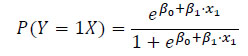
The logistic regression model is based on a logistic function that can be expressed as follows [13]:
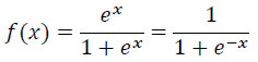 |
When e represents the Euler number and x represents the value of the explanatory variable X. Depending on the determined value, it can be written in a variety of ways. If the probability of success is estimated (assuming Y is a dichotomous variable with values of 1) for the occurrence of the event of interest (success) and 0 for the opposite case (failure), the logistic regression model is defined by the equation:
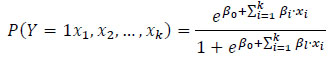 |
where βi i = 0, . . ., k are logistic regression coefficients, x1, x2, . . ., xk – independent variables, which can be both measurable and qualitative. Logistic regression can also be understood in terms of the probability of the event being examined occurring (success):
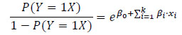 |
The probabilities are calculated by dividing the likelihood of an event happening P(A) by the probability of an event not happening 1 − P(A):
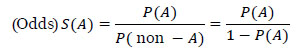 |
The logistic regression equation looks such as this when there is only one independent variable:
 |
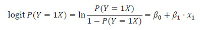
Logit form of the logistic model could be obtained by logarithmizing both sides of the equation:
 |
The logistic regression model has its own set of criteria. Its application is constrained by the test sample size, which must be more than or equal to n > 10(k + 1), where k is the number of predictors.
In this article, the binary logit model is selected as the basic model. The maximum likelihood (ML) technique, which maximizes the probability of classifying the observed data into the right category given the regression coefficients, is used to create the best-fitting function in logistic regression. For the structural portion of the utility function, the general formulation is:
 |
where:
- β are the coefficients to be estimated.
- Travel cost and travel time are the variables associated with travel cost and travel time, respectively.
- Ɛ other illustrating parameters in the model.
- The utility function is unitless.
The cost coefficient and the time coefficient capture the sensitivity of the passengers in adjusting the time of travel and the cost. Thus, their ratio should be used for exchanging time and transport costs; in other words, VOT. Please check the formulation below for more details:
 |
The coefficient ratio of the time of travel over the travel cost coefficient will lead to a result in pounds/minute (or in pounds/HR. when multiplied by 60).
5. SURVEY DESIGN DATA
The data collected may either be emanated data from revealed preferences (RP) or stated preferences (SP). RP data reflect the individual travelers' actions and can be collected through polls and field studies. The SP data is the traveler’s behavior, which can be derived from SP surveys and simulators in hypothetical scenarios.
There were three sections of the questionnaire.
The first element intends to gather the individual's socio-economic results. The second section gives information about the recent journey on a typical day. As for the third part, the stated preference SP of a given choice is compiled. Responses in the form of “choice” among the presented choice alternatives were utilized to develop utility models and the estimated coefficients from the developed models were used to estimate VOT measures. The quantitative attributes such as travel time and travel cost were considered for the preparation of alternatives. A major consideration in selecting attribute levels is the range and degree of variation. Four levels were considered for each attribute. Attributes and the corresponding levels used in the experiment are given in Table 1.
The survey of the interviewees’ samples was altered over eight weeks. The survey sample was chosen in light of the population of the residents in Egypt using Google Forms, where respondents need to be signed into their Google accounts before they can reply. Several questionnaires were also obtained via interviews; 1123 from a total of 1370 analyzable selected respondents. The specification of the questionnaire used in the experiment and the preliminary analysis overview statistics are shown in Table 2.
| Attributes | Level 1 | Level 2 | Level 3 | Level 4 |
| Travel time in minutes | Remain the same | Reduced by 15% | Reduced by 25% | Reduced by 35% |
| Travel cost in pounds | Remain the same | Increased by 20% | Increased by 40% | Increased by 80% |
The data has been coded for several levels to get a comprehensive evaluation of each attribute. Some variables are categorized into two levels, such as gender (i.e., Male = 0 & Female = 1), while other variables were classified into five levels, such as age (years) and the length of the trip. Some levels indicate concepts that cannot be coded like ‘Others’. Therefore, the analysis purposes levels which have the same concepts were combined into one level or blotted out as the software is capable of dealing with the coded data only.
The preliminary research clarified that gender seems to be equal since 49.9% are males and 50.1% are females. Modal split showed that 43.5% of surveyed people choose public transportation and 47.6% choose Private cars for their trips. It is observed that 62.2% of trips are Work trips.
| Parts* | Ranges | Percentage% |
| Part (1) Socio-economic Details | Male Female |
49.9% 50.1% |
| Married Unmarried Others |
62.8% 34.7% 2.5% |
|
| 18-25 25-35 35-45 45-60 >60 |
20.6% 54% 16.8% 6.3% 2.3% |
|
| Without Medium Above medium High Above High |
0% 8.6% 24.7% 56.7% 10% |
|
| 0-2000 2000-4000 4000-10000 10000-15000 >15000 |
29.5% 27.5% 26.5% 7.4% 9.1% |
|
| Unemployed Government emp. Private emp. Public sector Free business |
25.7% 2.1% 38.7% 22.4% 11.1% |
|
| Part (2) Trip Details | Work Study Entertaining Shopping Others |
62.6% 11.1% 9.7% 10.9% 2.1% |
| Private car Public transportation Others |
47.6% 43.5% 9.1% |
|
| 0-10 10-20 20-35 35-50 >50 |
12.2% 14.7% 17.5 % 22.2% 33.4% |
|
| written by the respondent | Max.=720 Min.=4 |
|
| written by the respondent | Max.=700 Min.=2 |
|
| Part (3) Stated Preference | 0.85 TT1, 1.2 TC1 0.80 TT1, 1.4 TC1 0.65 TT1, 1.8 TC1 TT1& TC1 remain the same |
68.40% 18.18% 10.22% 3.2% |
6. MODEL ESTIMATION
In a variety of public transport policy and planning applications, Value of Time (VOT) initiatives are valuable. Nevertheless, VOT is a latent variable that cannot be directly calculated. As a consequence, methodologies have been established for the indirect measurement of the VOT.
6.1. Binary Logistic Regression
The binary logistic regression model is used to analyze binary outcome variables. It also makes use of the relationship between independent variables and dependent (or outcome) variables that is discrete. This model can be used to investigate the impact of a certain exposure on a variety of outcome variables, such as:
- Comparing the level of an outcome variable in two exposure groups
- Comparing more than two exposure groups through the use of indicator variables to estimate the effect of different levels of a categorical variable compared to a baseline.
6.2. Mode of Travel Cross Classification
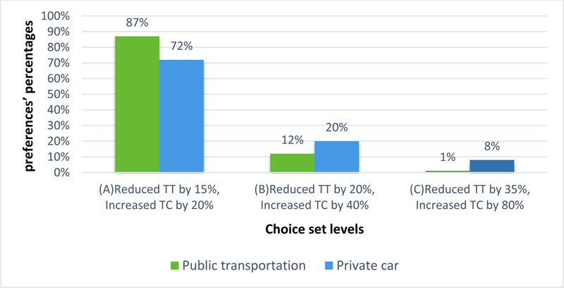
The transportation service is considered one of the most important elements that enhance the development of any country due to the significant role of transportation in many aspects such as the social and the economic ones. Therefore, transportation planners need to control the modal split between available modes of transport and promote particular modes such as public transport, walking, and cycling. The different preferences percentages of each respondent for each available mode of transportation are shown in Fig. (1).
In the previous figure, it can be seen that private car owners have more willingness than public transport users to pay money to save time. However, reducing the travel time by 15% remains the highest preference for the users of each mode and that increased the travel cost by 20%. The study was limited to private cars and public transportation only because they are the most widely used vehicles for urban traveling in Egypt; other modes like walking and cycling are not common.
Binary logistic regression is used to evaluate travel cost and travel time coefficients, to measure VOT. The models were calibrated separately for private cars and public transportation modes. All the variables presented in Table 3 have significant parameter estimates and logical signs.
The logistic regression model is statistically significant when p is < or = 0.05. For the statistical significance of the test asterisk* and ** have been used for significance values. As an example, Travel time* (p = 0.021) (p =0.008), Travel cost* (p = 0.004) (p = 0.032), for private car and public transportation were respectively added significantly to the model. The coefficient estimates for evaluating VOT and several variables were evaluated during the calibration process, the statistical test used is presented in Table 4.
The Hosmer-Lemeshow test the null hypothesis that the predictions made by the model fit perfectly with the observed group memberships. A chi-square statistic is computed comparing the observed frequencies with those expected under the linear model. A non-significant chi-square (p = 0.85) for private cars and (p=0.70) for public transportation indicates that the data fit the model well.
Cox & Snell R Square and Nagelkerke R Square values are methods of calculating the explained variation. These values are sometimes referred to as (pseudo R2) values. Therefore, the explained variation in the dependent variable, which was based on private cars, ranges from 24.0% to 33.0%, and 30.0% to 38.0% for public transportation.
| - | Variable | Private Car | Public Transportation | |
| Coefficient | Coefficient | |||
| - | Travel Time TT(min)* | 0.0231 | 0.0493 | |
| Travel Cost TC(pound)* | 0.0426 | 0.1606 | ||
| Trip Details | Trip purpose** | Work Study Entertaining |
0.451 1.271 0.547 |
1.558 0.359 1.822 |
| Trip length** (km) | 0-10 10-20 20-35 35-50 |
0.910 0.553 1.648 0.442 |
0.777 0.345 1.493 0.782 |
|
| Socio-economic Details | Gender** | Gender | 0.772 | 0.990 |
| Age** ( years) |
18-25 25-35 35-45 45-60 |
2.567 0.487 1.298 0.434 |
1.298 0.545 0.123 1.287 |
|
| Marital status** | Married Unmarried |
0.755 0.877 |
17360. 0.372 |
|
| Education level** | Without Medium Above med. High |
0.410 1.565 0.607 0.589 |
0.690 0.597 1.217 0.142 |
|
| Occupation** | Unemployed Government Private emp. Public sector |
0.229 0.971 0.461 0.459 |
0.148 0.279 0.093 0.705 |
|
| Monthly income* (pound) | 0-4000 4000-10000 |
0.943 0.866 |
1.0700 0.523 |
|
** non-significant p> 0.05.
Table 4.
| Statistical Test | Private Car | Public Transportation |
| Chi-square sig. | 0.85 | 0.70 |
| Cox & Snell R Square | 0.2454 | 0.3063 |
| Nagelkerke R Square | 0.3375 | 0.3821 |
| VOT (LE/hr) | 32.5 | 18.3 |
| VOT ($/hr) | 2.07 | 1.17 |
Variation in VOT between the private car (32.5 LE/HR.) and public transportation (18.3 LE/HR.) is based on the intuition of the vehicle owners’ that they can control time and choose their travel path, which is indeed not available for public transportation users.
6.3. Personal Monthly Income Cross Classification
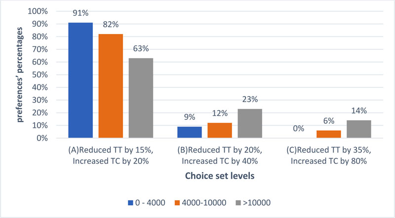
The average wage rate is recommended as a basis for determining the value of time unless reliable information on the earnings of users of transportation is available. Both theoretical and empirical research indicate that the value of time can be significantly higher or lower than the current wage rate; depending on the activities people are involved in [14]. Therefore, in this research, various classes of income, such as the variance of VOT, could be interpreted. The coefficient estimates for various income levels using binary logit models and VOT values are shown in Table 3, and preferences’ percentages of different personal monthly income levels are shown in Fig. (2).
The previous figure showed that the travelers’ willingness to pay for saving time increases when their income increases. This is logical because travelers aim to save time and arrive at their destination as soon as possible; however, the available budget restricts their decision. As seen in the table below, the first choice set level (A) – reduced the travel time by 15%, and increased the travel cost by 20% - and that is why this choice was the most preferable one for all the monthly income groups. This could also be considered a reflection of a certain socio-economic condition. Furthermore, binary logit analysis is applied in Table 5 to estimate VOT for each personal monthly income group separately.
The traveler’s travel time, travel cost, and occupation are the most significant variables in all the monthly income models. The negative coefficient for travel time and travel cost indicates the decreased utility associated with the increased travel time and travel cost. The traveler’s occupation is logically significant as the expected income and the responsibilities of the higher-level employees are much more than that of the lower-level employees. The calibration process and the statistical test used are shown in Table 6.
As previously mentioned, the travelers’ VOT increases when their income increases. VOT variation ranges between 13.5 LE/HR and 89.4 LE/HR. A non-significant chi-square for all monthly income levels (p> 0.05) indicates that the data fit the model well. The explained variation in the dependent variable, which was based on monthly income level, ranges from 35.4% to 37.8% for monthly income between (0-4000), ranges from 25.6% to 48.1%, and 39.5% to 11.1% for monthly income between (4000 – 10000) and >10000 respectively.
| Variable | 0 - 4000 | 4000 – 10000 | >10000 | ||
| Coefficient | Coefficient | Coefficient | |||
| * Travel Time TT(min) | -0.024 | -0.077 | -0.088 | ||
| Travel Cost TC(pound)* | -0.106 | -0.110 | -0.059 | ||
| Trip Details | Trip purpose** | Work Study Entertaining |
0.119 2.286 0.198 |
0.235 0.770 1.441 |
0.535 1. 494 0.666 |
| Trip length** (km) | 0-10 10-20 20-35 35-50 |
1. 830 0.686 1.385 0.713 |
0.461 0.512 0.837 0.324 |
0.913 0.690 0.150 2. 225 |
|
| Mode of travel** | Private car Public transportation |
0.585 0.087 |
0.178 0.053 |
0.905 0.261 |
|
| Socio-economic Details | Gender** | gender | 0.939 | 0.175 | 0.927 |
| Age** ( years) |
18-25 25-35 35-45 45-60 |
1. 060 0.913 0.293 1. 807 |
0.235 0.933 0.833 1. 315 |
0.849 1. 675 0.892 0.275 |
|
| Marital status** | Married Unmarried |
0.500 0.525 |
0.235 0.736 |
0.664 0.315 |
|
| Occupation* | Unemployed Government Private emp. Public sector |
1.824 0.983 0.508 2.207 |
0.805 2.129 0.052 0.910 |
0.411 1.614 0.831 1. 203 |
|
| Education level** | Without Medium Above Med High |
0.195 1. 074 0.897 0.151 |
0.550 0.369 0.405 1. 686 |
1. 079 0.267 0.442 0.915 |
|
** non-significant p> 0.05.
| Statistical Test | 0 - 4000 | 4000 – 10000 | >10000 |
| Chi-square sig. | 0.139 | 0.175 | 0.564 |
| Cox & Snell R Square | 0.354 | 0.256 | 0.395 |
| Nagelkerke R Square | 0.378 | 0.481 | 0.111 |
| VOT (LE/hr) | 13.5 | 42.0 | 89.4 |
| VOT ($/hr) | 0.86 | 2.68 | 5.69 |
6.4. Trip Purpose Cross Classification
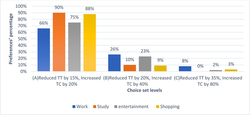
The purpose of a trip greatly influences the traveler’s behavior and mode choice. The figure below is designed to depict four major trip purposes which are: work/business, Study, entertainment, and shopping. All of these activities are relevant to a normal typical day. Work/business trips seem to be the most frequent activity, 62%, compared to the other ones because it is a common regular trip for many people. The preferences’ percentage of different trips’ purposes is shown in Fig. (3).
From the figure above, it can be noticed that the traveler’s willingness to pay is higher for work/business trips than the other trips, and this happens because work trips are restricted by certain attendance and departure times and each job has different responsibilities. As for the study-related trips, its travelers show less willingness to pay and this may occur because of the limited income of the students. As for leisure trips, it is found that the travelers’ desire to pay increases as they aim to reduce the time they spent on reaching their destination. In other words, these travelers would certainly pay as much money as needed to save any wasted time on the road trips, especially since most of the trips take a long time because of the long distance (Table 7).
As Tables 3, 5, and 7 above show, travel time and travel cost are the most significant variables in all binary trip purpose models. Values of travel time for different trip purposes are given in Table 8.
| Variable | Work | Study | Entertaining | Shopping | ||
| Coefficient | Coefficient | Coefficient | Coefficient | |||
| Trip Details | Travel Time TT(min)* | 0.011 | 0.198 | 0.023 | 0.035 | |
| Travel Cost TC(pound)* | 0.017 | 0.621 | 0.045 | 0.087 | ||
| Trip length** (km) | 0-10 10-20 20-35 35-50 |
0.610 0.919 0.314 0.606 |
0.610 0.68 0.09 0.919 |
0.933 0.729 0.719 0.882 |
0.606 0.704 0.406 0.627 |
|
| Mode of travel** | Private car Public transportation |
0.710 0.275 |
0.021 0.76 |
0.566 0.848 |
0.369 0.055 |
|
| Socio-economic Details | Gender** | gender | 0.604 | 0.141 | 0.744 | 0.335 |
| Age** ( years) |
18-25 25-35 35-45 45-60 |
0.537 0.701 0.239 0.688 |
0.610 0.919 0.314 0.26 |
0.933 0.729 0.719 0.882 |
0.606 0.704 0.406 0.627 |
|
| Marital status** | Married Unmarried |
0.934 0.596 |
0.46 0.36 |
0.709 0.532 |
0.413 0.328 |
|
| Education level** | Without Medium Above Med. High |
0.338 0.105 0.378 0.777 |
0.76 0.142 0.910 0.73 |
0.961 0.427 0.049 0.514 |
0.641 0.033 0.690 0.640 |
|
| Occupation** | Unemployed Government Private emp. Public sector |
0.738 0.850 0.812 0.967 |
0.00 0.28 0.63 0.32 |
0.294 0.931 0.559 0.708 |
0.187 0.198 0.956 0.952 |
|
| Personal monthly income** (pound) | 0-4000 4000-10000 |
0.471 0.435 |
0.415 0.20 |
0.408 0.929 |
0.127 0.140 |
|
** non-significant p> 0.05.
| Statistical Test | Work | Study | Entertaining | Shopping |
| Chi-square sig. | 0.127 | 0.251 | 0.156 | 0.114 |
| Cox & Snell R Square | 0.252 | 0.176 | 0.342 | 0.426 |
| Nagelkerke R Square | 0.389 | 0.537 | 0.474 | 0.191 |
| VOT (LE/hr) | 38.82 | 19.15 | 30.66 | 24.13 |
| VOT ($/hr) | 2.47 | 1.22 | 1.95 | 1.54 |
| Public Transportation | Private Car | Mode of Travel | ||||
| >10000 | 4000-10000 | 0-4000 | >10000 | 4000-10000 | 0-4000 | Income level (pound) |
| 30.62 | 24.50 | 15.33 | 81.30 | 55.42 | 31.23 | Work trip |
| 12.36 | 10.64 | 8.80 | 20.44 | 17.13 | 15.78 | study trip |
| 24.24 | 20.13 | 13.57 | 66.65 | 39.54 | 25.43 | Entertaining trip |
| 21.0 | 14.43 | 10.66 | 42.59 | 26.87 | 20.54 | Shopping trip |
A non-significant chi-square value represents an acceptable model fit. Cox, Snell R Square, and Nagelkerke R Square values of all the models lie between 17% and 53%. The Value of Travel Time varies according to the purpose of the trip; the highest VOT, 38.82 LE/HR, was found on business-oriented trips.
7. RESULTS AND DISCUSSIONS
The value of travel time (VOT) is an important input to travel demand modelsand is used to manage and evaluate transportation investment decisions [15, 16]. This paper provides an estimation of the value of travel time using a combined RP-SP method. The analysis is undertaken to achieve the following objectives; I) defining the required methods for estimating the value of travel time depending on the expanded literature review; ii) measuring the value of travel time for private cars and public transportation modes within different income levels and several trip purposes; and iii) finding out the effect Cross classification of socio-economic factors on the travel time value.
Travel time values are critical in the design of transportation infrastructure. In transportation models, the value of time is utilized to commercialize travel time based on the socioeconomic status of travelers. Providing improved travel time is generally among the largest societal benefits of transportation infrastructure projects. Table 9 gives the VOT for different travel experiences in Egypt.
This paper assesses the estimation of the value of time-based on questionnaires distributed to travelers in a preference survey. The findings of this study aim to help researchers and practitioners to explore the applicability of binary logic regression in modeling the value of travel time using combined stated and revealed preference survey data.
Accurate traveler VOT calculations aid in determining the potential worth of such costs/benefits about the required monetary expenditure. Savings in travel time can also result in lower vehicle running expenses. The association between trip duration and reliability is established by [17] establish the relationship between travel time and reliability. This relationship is useful to find the value of reliability savings by improving the network in a case study.
CONCLUSION
The findings revealed that various socioeconomic demographic variables and trip parameters all played a role in varying degrees of VOT variances. It aids in a better understanding of which characteristics contribute to higher or lower VOT and to what extent.
These findings can be included in the demand forecasting process, resulting in more accurate estimates and analytical capabilities in a variety of applications, including toll feasibility studies, pricing strategy, policy evaluations, and impact analyses.
Finally, the binary logit technique appears to be the most appropriate method for estimating the value of travel time (VOT), as it is an accurate, dependable, straightforward, and broadly applicable logistic regression model.
It is hoped that this study has proved the binary logit model's relevance to the cross-classified Value of Time and that it will be widely used in Egypt soon. It is suggested that more research be done to examine the impact of social and economic factors on the value of travel time for trips of varying lengths and people with occupations other than those listed in this study. Different logistic regression models can also be used to undertake other investigations.
LIST OF ABBREVIATIONS
| VOT | = Value of Travel Time |
| RP | = Revealed Preference |
| SP | = Stated Preference |
| VTTS | = Value of Travel Time Savings |
| VAT | = Value of Time Assigned to Travel |
CONSENT FOR PUBLICATION
Not applicable.
AVAILABILITY OF DATA AND MATERIALS
The data that support the findings of this study are available within the article.
FUNDING
None.
CONFLICT OF INTEREST
The authors declare no conflict of interest, financial or otherwise.
ACKNOWLEDGEMENTS
Declared none.

