All published articles of this journal are available on ScienceDirect.

Modelling Mixed Traffic Time Headway Distribution Induced by Bus Rapid Transit (BRT) in Cape Town, South Africa
Abstract
Background:
The safety and capacity of roadways are immensely influenced by time headways, a major traffic flow characteristic. Time headways are frequently utilized in various aspects of traffic and transportation engineering studies, including capacity analyses, studies of safety, modelling of lane-changing and car-following behaviour, and level of service assessment.
Time headway, measured in seconds, refers to the distance between two subsequent passing cars moving over a single spot on the road. This paper reports the statistical modelling of the time headway distribution of a mixed traffic flow scenario caused by BRT via statistical headway distribution models. The paper posits that the introduction of BRT dedicated lane and its adopted design configuration induces anomalous traffic flows on its adjoining lanes with attendant time headway differentials, irrespective of the type of adopted design configuration for the corridor. The objectives of this study were to fit the BRT-induced time headway distribution to probability distribution models and determine the most appropriate distribution model that fits the data derived using the goodness of fit tests. Consequently, this contribution, therefore, fills the gap in research with respect to determining the precise model that fits the time headway distribution of mixed traffic flow scenarios induced by BRT.
Methods:
The time headway distribution data collected at four designated road segments on a multilane provincial route R27 caused by BRT dedicated lane in Cape Town, South Africa, were fitted to five probability distribution models viz, Lognormal, Inverse Gaussian, Log-logistic, Generalized Extreme Value (GEV), and Burr using MATLAB software. The fitted headway data were with respect to the traffic flows on the adjoining lanes to BRT or traffic flow ‘without BRT’. Precisely, the empirical data were collected over a three-month period using an Automatic Traffic Counter (ATC). Using ModelRisk software, the goodness of fit of the probability models was assessed by the Akaike Information Criterion (AIC), the Schwartz or Bayesian Information Criterion (SIC or BIC), the Hannan Quinn Information Criterion (HQIC), and the loglikelihood (LLH) model performance criteria respectively. The distribution model with the lowest AIC criterion and largest loglikelihood (LLH) values describe the model that best fits the headway data across the four sites.
Results:
Results showed that the models fitted the headway data well at each site by visual inspection of the attendant Probability Density Function (PDF) and the Probability plots (P-P). However, the Burr distribution provided the overall best fit based on the AIC and LLH values at 95% confidence and 0.05 significance levels across the four sites. At sites 02, 03, and 04, it ranked first with the lowest AIC values of 4025.99, 2595.56, 3815.36, and corresponding largest LLH values of -2008.98, -1293.76, and -1903.66, respectively, while the lognormal distribution performed best at site 01, with AIC value of 4445.14 and LLH value of -2220.57, closely followed by the Burr distribution with AIC and LLH values of 4453.05 and -2222.51, respectively. The P-values, which ranged between 0.65 and 0.80, showed the likelihood of the occurrence of the data sets under the null hypothesis. Hence the null hypothesis was accepted.
Conclusion:
The study concluded that the introduction of BRT dedicated lanes affects the adjoining lanes’ mixed traffic time headways’ distribution, and the headways are continuously distributed, hence fitting continuous probability distributions.
1. INTRODUCTION
According to the Highway Capacity Manual (HCM) 2010, time headway refers to “the time between two successive vehicles as they pass a point on a lane or roadway, measured in seconds from the same point on each vehicle” [1]. Time headway in traffic flow modelling and planning is considered a relevant control parameter that affects the behaviour of drivers, and it particularly plays a major role in the estimation of roadway capacity [2]. Time headway is a microscopic characteristic of flow that has also found useful applications in the estimation of Passenger Car Units (PCUs), Level of Service (LOS) evaluation, analysis of safety, gap acceptance studies, and delay studies [3, 4] It is a fundamental characteristic of the quality and quantity of traffic flow [5], that describes the order in which a leading car and the one that follows it arrive at selected points on a roadway [6]. Its analysis has been found to be one of the most important methods in traffic engineering, employed to understand the position of one vehicle relative to the other in a mixed traffic flow [6]. In terms of quantitative applications, it is inversely proportional to capacity and traffic volume. Furthermore, it has significant usage in traffic simulations, merge-diverge decisions of drivers at intersections, and traffic safety analysis [7]. The concept of traffic flow is particularly an overly complex and tricky phenomenon that is difficult to understand. However, headway analysis through stochastic models has been found to be able to explain it to some extent. It is, therefore, not a wonder that several attempts have been made to develop models that can explain the headway distribution under different prevailing conditions. The modelling of time headways involves the description of how the traffic stream behaves by paying close attention to the characteristics of the individual vehicles. There are several applications of time headway models, with attendant merits and demerits. Time headway models are often used to study vehicle spacing and analyse the arrival rates of vehicles at a given point or location of an accident during accident studies. By carefully modelling and analysing the distribution of vehicle headways, traffic engineers can increase route capacity and decrease vehicle delay [8]. In terms of safety, the decision drivers make to either merge, pass, weave, or just follow a leading vehicle is a function of their perception of a safe time headway between them and the other vehicles in their vicinity. Time headway modelling is also employed to investigate the pattern with which traffic fluctuates within an interval of time and the possibility of congestion. Additionally, headway distributions are required for digital simulations that use driving simulators to simulate multilane traffic [8]. Additionally, headway analysis makes it possible to learn more about the causes of collisions and strategies for enhancing traffic safety. In capacity modeling, the safety headway requirement is often ignored during model calibration and parameter estimates. This could help to partially explain why some issues frequently arise on roads carrying less traffic than their theoretical capacity [9].
Mixed traffic flows on roadways are characterized by incessant traffic manoeuvres, speed changes, and weak lane discipline, amongst other anomalous behaviours in the stream. The presence of vehicles of different sizes, varied manoeuvrability, and dynamic features often lead to differential in-vehicle time headways varying from zero to several seconds [6]. These characteristics result in transportation burdens, such as delay, platooning, and traffic jams as soon as the jam density is reached and all vehicles come to a stop. Mixed traffic flows on the adjoining lanes to a BRT dedicated lane are not an exception to these problems, but there has been limited literature that has investigated this scenario, despite several previous studies on heterogeneous traffic time headways. Given this situation, this study, therefore, analyzes the headway data collected at four different road segments in Cape Town, South Africa, and explores the possibility of fitting the headway data to probability distribution models, as well as determining the distribution that best fits the headway distribution caused by BRT. This further helps to understand the attendant anomalous changes in traffic characteristics, such as time headways, due to physical roadway constraints, such as BRT dedicated lanes, through stochastic models.
2. LITERATURE REVIEW
2.1. Time Headway Distribution on Roadways and Freeways
Time headway distributions on roadways and freeways have been previously studied and documented in the literature. In 1993, Mei and Bullen investigated the number of headways measured on two southbound lanes of a four-lane motorway during the morning rush hour through probability distribution models. The lognormal distribution was the optimum model for the time headways in heavy traffic flow at both specified lanes, which was found to be with a 0.3 or 0.4 second shifting. In a study by [10] on interstate highways in Illinois, the United States, headways were recorded at traffic rates ranging from 140 to 1704 vehicles per hour per lane. The study recommended generating the time headway distribution for any traffic volume for both the right and left lanes using the lognormal model with a shift of 0.36 seconds. Thamizh [11] looked at the time headway data gathered from a divided urban arterial in Chennai City, India, with four lanes. It was discovered that the negative exponential statistical distribution could accurately simulate headways for all traffic flows and lane configurations. Bham and Ancha [12] also studied the temporal car-following headways for several sorts of highway sections in a steady state. A standard highway segment, lane shift, ramp merge, along with ramp weave part are all present at the data sites. In comparison to the shifted gamma distribution, the lognormal distribution with shifts was found to offer a superior fit for each of the locations cited. In Riyadh, Saudi Arabia, Al-Ghamdi [12] examined time headways observed on urban highways. Three categories of traffic flow were used to categorize the observed vehicle flow range: low (400 vehicles per hr), medium (400–1200 vehicles per hr), and high (>1200 vehicles per hr). His analysis found Erlang, shifted-exponential, and negative exponential distributions to be the best models.
He also noted that low-traffic situations had been the focus of the majority of the headway distribution studies that have been conducted. At large levels of traffic flow, the headway distribution modeling is nevertheless still hazy. Vehicle headways gathered from Finnish rural roadways were thoroughly analyzed by [13]. He concluded that low to moderate traffic levels with a low possibility of having short headways can be handled by the gamma distribution. Additionally, he asserted that the lognormal distribution could serve as a model for the follower headway distribution even though it is neither straightforward nor sufficiently realistic [13]. Zwahlen et al. [8], in 2007, studied the portability of the Ohio traffic load and lane traffic cumulative headway distributions. The study's findings demonstrated that for similar hourly traffic numbers, and for the most part, the headway distributions are the same for each lane. To examine the influence of specific factors on the time headway distribution, [15] used a synthetic Erlang distribution model to analyze headway data from multiple Japan-based sites. Besides, they looked for a law that relates to the model parameters. Results showed that each lane had a distinct background that could influence the distribution of time headways. Vehicle time headway distributions at varying flow rates on two- and four-lane roadways in India were examined by the researchers mentioned in the reference [6] using lognormal and log-Pearson statistical modelling methods. They also accessed the changes in the time headways of vehicles for several two-lane and four-lane routes throughout the morning and evening hours with mixed traffic. Their results not only captured the differences in headway distribution but also identified the headways of some types of vehicles, including the way vehicles maintain headways when headlights are turned on. In another study conducted in India by [14], the distribution of speed and time headway of vehicles in mixed vehicular traffic on four two-lane bidirectional roadways was examined using leader-follower vehicle pairs. Results showed that the speed and time headway distributions varied significantly and were found to have useful applications in capacity estimation, Level of Service (LOS) analysis, and the development of micro-simulation models. Time headway distributions were also modelled using three different probabilistic models (single, combined and mixed) by [15] in France. Results showed that the mixed models provided the best fit among several time headway samples. Using a traffic detector incorporated with laser sensors for sorting and analysis, the theoretical traffic flow models to analyse time headway distributions were developed, as mentioned in the reference [16]. The results gave a better understanding of headway in signalized arterials. In another study, [19] examined the impact of lane position on time headway in Isfahan, Iran, to evaluate driving behaviour at various highway lanes using headway distribution analysis. The results showed that the appropriate model for passing lanes differs from the one for middle lanes due to the different behavioural operations of drivers. In a study conducted by [17], time headway considering lateral distance was studied on a non-lane-based traffic flow using a novel approach, where time headways were divided into 5 intervals in form of a measuring criterion to evaluate time headway values and implications as “Unsafe (0-0.7 sec), non-lane-based car-following (0.9 sec), lane-based car-following (1.0 sec), overtaking time headway (1.3 sec), and free driving (larger than 2.5 sec)” [17]. Results indicated that “to differentiate between following and free-wheeling driving behavior, a reasonable criterion to use is the time headway of the overtaking operation”. Another closely related study conducted in China by [18] investigated traffic congestion and lane-changing patterns involving interactions between BRT and general traffic flow at a typical bottleneck along a BRT corridor. Results revealed abnormal lane violations resulting in a 16% reduction in the saturation rate of general traffic and 17% in bus travel time. Most of the studies discussed so far which have examined the time headway distributions of low, medium, and heavy mixed traffic flows were performed based on headway data of roadways or corridors without BRT dedicated lanes. The purpose of this paper is to report on the findings from a study that looked at how the presence of a BRT dedicated lane affected the time headway distribution of the high volume of mixed traffic that resulted on the adjoining lanes. The main thrust is to fit the headway data to probability distribution models and determine the most appropriate headway distribution model that best fits the data and the condition.
2.2. Hypothesis Testing and Estimation of Model Parameters
The technique known as “goodness of fit” is used to confirm and determine whether a probability distribution is suitable for simulating a specific phenomenon. The Akaike Information Criterion (AIC), the Schwartz or Bayesian Information Criterion (SIC or BIC), and the Hannan Quinn Information Criterion (HQIC) were the methodologies used in this investigation. Although the Chi-Squared (C-S), Kolmogorov-Smirnoff (K-S), and Anderson-Darling (A-D) goodness-of-fit statistics are still widely used today, they are not theoretically the best ways to compare distributions fit data. They cannot include censored, truncated, or binned data and are also restricted to accurate observations. The AIC, SIC, or BIC and HQIC, however, are statistical measures of fit generally known as information criteria. They are defined as follows:
A. AIC (Akaike Information Criterion): The Akaike Information Criterion is defined by the following model equation:
 |
(1) |
B. SIC (Schwarz Information Criterion, aka Bayesian Information Criterion BIC): The Schwarz Information Criterion, aka Bayesian Information Criterion, is defined as follows:
 |
(2) |
C. HQIC (Hannan-Quinn Information Criterion): The Hannan-Quinn Information Criterion is defined as follows:
 |
(3) |
The objective is to identify the model with the lowest information criterion value. Each formula has the -2ln [Lmax] term, which is an estimation of the model fit's deviation. Each formula's first component contains coefficients for k that indicate the severity of the penalty for the number of model parameters. Regarding punishing the loss of a degree of freedom, SIC [19] and HQIC [20] are stricter than AIC [21]. These three criteria are used to score each fitted model, whether it fits a copula, a time series model, or a distribution. Therefore, based on Maximum Likelihood Estimation (MLE), the model criterion with the lowest value of AIC, SIC, or BIC and HQIC provides the best fit. Amongst the three information criteria, the AIC ranking determines the best-fitted distribution.
2.3. Data Survey
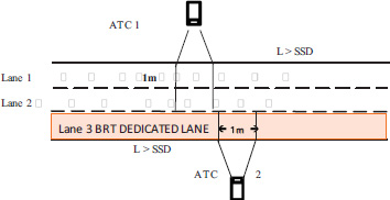
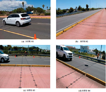
The data were collected in Cape Town, South Africa. Traffic Characteristics data of volume and speed were surveyed at four designated sites 01 – 04 along the BRT route R27 in Cape Town, South Africa, for a three-month period. The Automatic Traffic Counter (ATC), installed at the four sites, was used to collect the data 24 hours a day for the entire period. Each location utilized two ATC loggers, one of which recorded BRT traffic flow data on the BRT dedicated lane, while the other recorded data on the adjoining lanes. Fig. (1) shows the general layout of the impact study location. The multilane provincial trunk route BRT corridor, R27 in Cape Town, South Africa, was selected for the field data survey. The sites, which are located along the trunk route, were selected after satisfying the following location criteria: (1) the geometric feature of roadway under investigation had the presence of a BRT dedicated lane with median design configuration and two adjoining lanes lying in parallel to it; (2) the roadway segments had relatively flat topographical terrain void of steep vertical slopes that could affect the free flow speed data, as well as pavement surfaces free from defects, such as rutting and potholes etc.; (3) the roadway segments were free from the influence of road intersections, on-street parking, broken down vehicles, traffic police check points, roundabouts and fuel filling stations along the route, which could also affect the free flow of traffic; (4) the segment lengths were long enough to allow for the setting up of the survey equipment at spots where there was sufficient free flow speed and the segment length was greater than the stopping sight distance (SSD) to reduce or eliminate the effect of intersections. Each pneumatic tube was placed and connected to the ATC loggers in accordance with the specifications and configurations and nailed in both lanes 1m apart at the four sites, as shown in Fig. (2). The loggers identified three vehicle categories or classes viz: passenger car (PC), medium vehicles (MV), and heavy vehicle (HV). A total of about 4560 headways were extracted for all the sites from the individual vehicle characteristics data and sorted on a Microsoft Excel worksheet. Table 1 presents the descriptive statistical characteristics of the headways collected from each of the four sites surveyed. Between sites 01 and 03, the mean headway decreased, while site 04 experienced a significant increase. This is due to the low traffic volumes observed at site 04. The explanation for this is that the road segment mainly carries traffic volumes from this work. The standard deviation exhibited similar behaviour. The trend in the coefficient of variation indicates that there is a cluster of headways on the roadway segments, particularly at sections near intersections where long queues are formed at peak traffic quickly because the introduction of BRT dedicated lanes has eliminated one of the three previously available lanes, causing long queues to build up quickly. The time headway variable's positive skewness and kurtosis all indicate that most of the distribution's headways are to the left of the mean value, which suggests that the road segment may have smaller headways or isolated clusters.
3. MATERIALS AND METHODS
To analyze the observed time headway distribution of the mixed adjoining lanes traffic, the primary descriptive statistics of the data were determined first for each site, as shown in Table 2. Statistical models should be applied to fit time headway data, with the view of identifying or selecting a suitable model for time headway distribution. In this study, the off-peak time headway data of the mixed traffic flows on the adjoining lanes to BRT dedicated lanes, under steady flow conditions, were fitted to five probability distribution models using MATLAB software and were rated in the order in which they best fit the data. The fitted probability distribution models were the Lognormal, Log Logistic, Inverse Gaussian, Generalized Extreme Value (GEV), and Burr. ModelRisk, a Monte Carlo Simulation computer software was employed to perform the goodness of fit tests, targeted at determining the best and most appropriate distribution that fits the time headway data induced by BRT. The models are briefly discussed in the following section:
| Descriptive Statistics of Headways | SITE 01 | SITE 02 | SITE 03 | SITE 04 |
|---|---|---|---|---|
| Mean | 3,67 | 3,42 | 1,98 | 6,49 |
| Standard Error | 0,14 | 0,21 | 0,09 | 0,34 |
| Median | 2,1 | 1,5 | 1,3 | 2,1 |
| Mode | 1 | 1 | 1 | 1 |
| Standard Deviation | 4,55 | 6,50 | 3,67 | 11,05 |
| Sample Variance | 20,69 | 42,22 | 13,48 | 122,19 |
| Kurtosis | 13,00 | 23,09 | 86,68 | 7,53 |
| Skewness | 3,21 | 4,63 | 8,30 | 2,82 |
| Coefficient of Variance | 1,23 | 1,90 | 1,86 | 1,70 |
| Range | 37 | 50,4 | 60,1 | 58,7 |
| Minimum | 0 | 0 | 0 | 0 |
| Maximum | 37 | 50,4 | 60,1 | 58,7 |
| Sum | 3711 | 3382,7 | 3370,4 | 6797,1 |
| Sample Size | 1010 | 988 | 1705 | 1047 |
| SITES | Rank | ProbabilityModel | SIC | AIC | HQIC | LLH | P Value | Sig.Level | Hypo.Test | BestFit |
|---|---|---|---|---|---|---|---|---|---|---|
| SITE 01 | 1ST | Lognormal | 4454.97 | 4445.14 | 4448.87 | -2220.57 | 0.6939 | 0.050.050.050.050.05 | AcceptAcceptAcceptAcceptAccept | Lognormal |
| 2ND | InvGauss | 4463.79 | 4453.97 | 4457.69 | -2224.98 | 0.6553 | ||||
| 3RD | GEV | 4465.68 | 4450.95 | 4456.53 | -2222.46 | 0.7247 | ||||
| 4TH | Loglogistic | 4468.80 | 4458.97 | 4462.70 | -2227.48 | 0.7202 | ||||
| 5TH | Burr | 4472.68 | 4453.05 | 4460.48 | -2222.51 | 0.7248 | ||||
| SITE 02 | 2ND | GEV | 4042.28 | 4027.29 | 4032.96 | -2010.64 | 0.7832 | 0.050.050.050.050.05 | AcceptAcceptAcceptAcceptAccept | Burr |
| 1ST | Burr | 4045.97 | 4025.99 | 4033.52 | -2008.98 | 0.7872 | ||||
| 3RD | Loglogistic | 4086.84 | 4076.84 | 4080.62 | -2036.42 | 0.7962 | ||||
| 4TH | Lognormal | 4150.91 | 4140.91 | 4144.69 | -2068.45 | 0.7461 | ||||
| 5TH | InvGauss | 4162.53 | 4152.53 | 4156.30 | -2074.26 | 0.7055 | ||||
| SITE 03 | 1ST | Burr | 2614.86 | 2595.56 | 2602.89 | -1293.76 | 0.7642 | 0.050.050.050.050.05 | AcceptAcceptAcceptAcceptAccept | Burr |
| 2ND | GEV | 2631.74 | 2617.25 | 2622.76 | -1305.61 | 0.7578 | ||||
| 3RD | Loglogistic | 2654.73 | 2645.07 | 2648.75 | -1320.53 | 0.7667 | ||||
| 4TH | Lognormal | 2751.19 | 2741.53 | 2745.20 | -1368.76 | 0.7128 | ||||
| 5TH | InvGauss | 2808.83 | 2799.17 | 2802.85 | -1397.58 | 0.6621 | ||||
| SITE 04 | 2ND | GEV | 3834.77 | 3820.01 | 3825.60 | -1906.99 | 0.7854 | 0.050.050.050.050.05 | AcceptAcceptAcceptAcceptAccept | Burr |
| 1ST | Burr | 3835.04 | 3815.36 | 3822.81 | -1903.66 | 0.7919 | ||||
| 3RD | Loglogistic | 3866.87 | 3857.03 | 3860.76 | -1926.51 | 0.8036 | ||||
| 4TH | Lognormal | 3959.28 | 3949.43 | 3953.16 | -1972.71 | 0.7451 | ||||
| 5TH | InvGauss | 3976.94 | 3967.09 | 3970.82 | -1981.54 | 0.7028 |
3.1. Lognormal Distribution
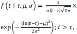
The well-known distribution model known as Lognormal is commonly employed in numerous research about headways. Additionally, modelling headways in instances where an automobile is followed is suggested by (Greenberg 1966). The mathematical expression for the lognormal distribution is:
 |
(4) |
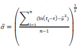
where: τ denotes the shift's value in seconds; µ and σ are the “location” and “scale” variables of the lognormal distribution, respectively. The following can be deduced from the observed data::
 |
(5) |
 |
(6) |
 |
(7) |
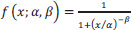
3.2. Log Logistic Distribution
The log-logistic distribution is non-negative random variable probability distribution that is continuous and whose logarithm has a logistic distribution. Although it has heavier tails, it has a comparable shape to the log-normal distribution. Its cumulative distribution function can be expressed in closed form, unlike the log-normal distribution. The probability density function of a log-logistic distribution can be expressed as:
Probability Density Function:
 |
(8) |
and the Cumulative Distribution Function:
 |
(9) |
Where x > 0, α > 0, β > 0
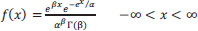
3.3. Inverse Gaussian Distribution
The inverse Gaussian distribution is a family of continuous probability distributions with two parameters that has support on (0, ∞). It shares numerous characteristics with a Gaussian distribution. While the Gaussian represents a Brownian motion's level at a defined time, the inverse Gaussian defines the distribution of the time it takes for a Brownian motion with positive drift to achieve a fixed positive level. The probability density function of the Inverse Gaussian Distribution is given by:
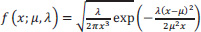 |
(10) |
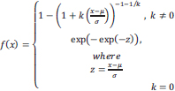
3.4. Generalized Extreme Value Distribution (GEV)
A family of continuous probability distributions known as the Generalized Extreme Value (GEV) was created from the extreme value theory. It serves as a limit distribution of correctly normalized maxima of a series of independent random variables with similar distributions. As a result, it is utilized as an approximation to describe the maxima of lengthy (finite) sequences of random variables. The distribution has a continuous scale parameter (k > 0) and a continuous shape parameter (k > 0). The PDF and CDF for this distribution are described as follows:
 |
(11) |
Cumulative Distribution Function:
 |
(12) |
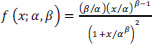
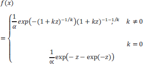
3.5. Burr Distribution
The Burr Distribution, also known as the generalized log-logistic distribution, is a continuous probability distribution for a non-negative random variable. To simulate household income, it is frequently utilized. Continuous shape parameters (k > 0; α > 0), continuous scale parameters (β > 0), and continuous location parameters (γ > 0) are present, and the PDF and CDF are given by:
Probability Density Function (PDF):
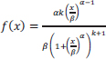 |
(13) |
Cumulative Distribution Function (CDF):
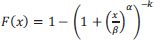 |
(14) |
To decide which of the distributions is the most appropriate model for headway data on each road segment, the five probability distribution models were subjected to goodness-of-fit tests earlier defined, also referred to as hypothesis testing. The following procedure was employed to select the best headway distribution model:
3.5.1. Step 1
The models were tested using the three goodness of fit criteria viz: AIC, SIC and HQIC, through the ModelRisk software.
3.5.2. Step 2
The generated AIC, SIC and HQIC goodness of fit values were observed on the software interface, and the models with the lowest AIC and largest LLH values for each site were located, which determined the best-fitted distribution.
3.5.3. Step 3
The generated model parameters viz shape, scale, and location were applied to determine the P-value. The higher the P-value and the more it exceeded 0.05 in all three tests at a 5 percent level of significance and 95% level of confidence, the more compatible the model.
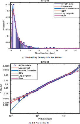
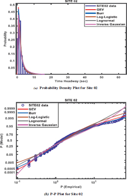
4. RESULTS AND DISCUSSION
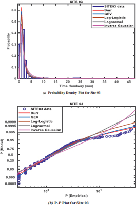
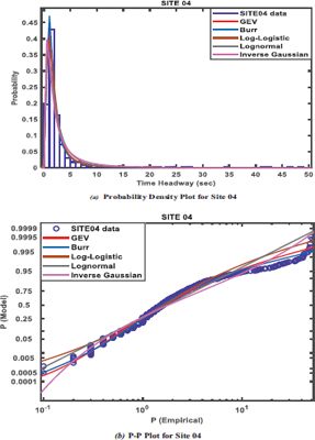
The study is based on the following hypotheses: (1) the compatibility of observed time headway distribution with the fitted probability distribution model is rejected if (p-value < α) or accepted (p-value > α), where α = 0.05 (2) the distribution which gives the smallest AIC, SIC and HQIC values, as well as the largest log-likelihood value is considered the best-fitted model [22, 23]. The information criterion that determines the overall best-performing distribution is the AIC. The five probability distributions earlier described were used to fit the time headway data surveyed from each site. The probability density function (PDF) or f(x) and p-p plots for each site, as shown in Fig. (3 to 6), indicate how well each distribution fits. All distributions fitted the headway data by visual inspection.
However, from the information criteria measures of the goodness of fit on the distributions as shown in Table 2, the Burr distribution provided the best fit with respect to the values of the Akaike Information Criterion (AIC), the Schwartz or Bayesian Information Criterion (SIC or BIC), and the Hannan Quinn Information Criterion (HQIC) at sites 02 – 04 at 95% level of confidence, and 0.05 level of significance, while the Lognormal distribution provided the best fit at site 01. Based on the postulated hypothesis, which states that the compatibility of observed time headway distribution with fitted probability distribution model is rejected if (p-value < α) or accepted (p-value > α), the fitted distributions were tested at 5% significance level (α = 0.05). Among the distribution with the lowest AIC value, and the largest LLH value to be selected as the distribution that provides the best fit, the Burr distribution emerged as the best-fitted and performed model, with the largest log-likelihood values of -2008, -1293.76, -1903.66, and lowest AIC values of 4025.99, 2595.56, and 3815.36, at sites 02, 03, and 04 respectively. This was followed by the lognormal distribution, which performed best at site 01 only, with the largest loglikelihood value of -2220.57 and the lowest AIC value of 4445.14. The P-values ranged between 0.65 and 0.80, and were greater than 0.05; hence they were acceptable based on the null hypothesis.
4.1. Parameters of the Probability Distribution
The distributions fitted to the time headways revealed varied estimated parameters, as shown in Table 3. Amongst these distributions, only the Lognormal, Inverse Gaussian, and Loglogistic have two parameters (shape and scale).
| Location | Probability Distribution | Shape Parameter | Scale Parameter | Location Parameter | |
|---|---|---|---|---|---|
| SITE 01 | Lognormal | 0.957653 | - | 0.824768 | - |
| InvGauss | 2.46774 | - | 3.68217 | - | |
| GEV | 0.587635 | - | 1.33665 | 0.0506121 | |
| LogLogistic | 0.544557 | - | 0.800605 | - | |
| Burr | 2.06566 | 0.745544 | 1.7652 | - | |
| SITE 02 | GEV | 0.627169 | - | 0.887089 | 1.12756 |
| Burr | 2.80529 | 0.462925 | 0.937949 | - | |
| LogLogistic | 0.517502 | - | 0.429871 | - | |
| Lognormal | 0.962479 | - | 0.498461 | - | |
| InvGauss | 1.75999 | - | 3.11653 | - | |
| SITE 03 | Burr | 3.14174 | 0.563195 | 0.951033 | - |
| GEV | 0.491284 | - | 0.631632 | 0.994844 | |
| LogLogistic | 0.407593 | - | 0.25756 | - | |
| Lognormal | 0.778561 | - | 0.302106 | - | |
| InvGauss | 2.09987 | - | 2.13115 | - | |
| SITE 04 | Burr | 2.84908 | 0.489718 | 1.07838 | - |
| GEV | 0.581184 | - | 0.950245 | 1.24518 | |
| LogLogistic | 0.492308 | - | 0.506001 | - | |
| Lognormal | 0.943592 | - | 0.576195 | - | |
| InvGauss | 1.9604 | 3.30588 | - | ||
The Burr and GEV distributions have three which are the shape, scale, and location parameters. Each of the parameters of the distribution varied in different proportions across the four sites. Their magnitudes and differentials were significant in all sites investigated.
CONCLUSION
This study examined continuous probability distributions to determine the most appropriate model that best fits the mixed traffic time headways on the adjoining lanes of the route R27 BRT dedicated lanes in Cape Town, South Africa. Five probability distribution models were fitted to the time headway data at each site, represented by PDF and P-P plots using MATLAB 2021 software. The goodness of fit of the probability models was assessed by the Akaike Information Criterion (AIC), the Schwartz or Bayesian Information Criterion (SIC or BIC), and the Hannan Quinn Information Criterion (HQIC) model performance criteria, respectively, using ModelRisk software. The probability distribution with the lowest AIC criterion and the largest loglikelihood (LLH) values was selected as the model that best fits the headways across the four sites. Based on the postulated hypothesis, the Burr distribution provided the overall best fit. This affirms the assertion in a study by [24] that the Burr distribution model is capable of modelling most time headway distributions under many prevailing conditions. The P- values were greater than 0.05. Hence the null hypothesis was accepted. Based on the results obtained, the following conclusions were drawn:
• The introduction of BRT dedicated lane results in a bottleneck in the flow of traffic on their adjoining lanes, characterized by speed drops and minimized time headways.
• The time headways are continuously distributed, fitting the selected continuous probability distributions.
• The time headway differentials are significant compared to the headway of BRT buses on their dedicated lanes, as investigated in a related paper to this study by [25].
• The time headway distribution caused by BRT shows the possible aberrant behaviour of drivers in a mixed traffic stream, as shown by the skewness of the data.
Although the introduction of BRT-dedicated lanes was justified in the study by A. E. Modupe and J. Ben-Edigbe [25], which examined the capacity utilization effects of introducing BRT-dedicated lanes; considering the time headways distribution investigated in this study, it would be appropriate to recommend that a mixed traffic scenario is constructed with BRT at some selected sections, especially areas prone to congestion along the corridor, and the time headway distribution should be analyzed with simulations where the potential behaviour of drivers and traffic characteristics in that scenario are necessary to understand. Perhaps the created mixed traffic scenario ‘with BRT’ could engender safer headways, unlike the anomalous mixed traffic flows ‘without BRT’ on the adjoining lanes caused by BRT, which threatens the safety of commuters and pedestrians.
LIST OF ABBREVIATIONS
| HQIC | = Hannan Quinn Information Criterion |
| LLH | = Log likelihood |
| AIC | = Akaike Information Criterion |
| SIC | = Schwarz Information Criterion |
| BIC | = Bayesian Information Criterion |
CONSENT FOR PUBLICATION
Not applicable.
AVAILABILITY OF DATA AND MATERIALS
The data and supportive information is available within the article
FUNDING
A three-year Ph.D. research grant with grant number 219091761 from the University of KwaZulu-Natal in Durban, South Africa, provided funding for this work.
CONFLICT OF INTEREST
The authors declare no conflict of interest, financial or otherwise.
ACKNOWLEDGEMENTS
The assistance of Mr. Sibusiso Ndebele and Prof. Mark Zuidgeest of the University of Cape Town during the data collection stage is highly appreciated.

